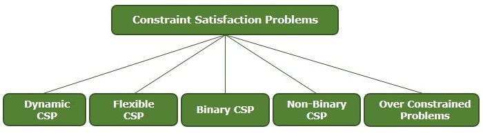
Artificial Intelligence - Types of CSPs

---

---

Constraint Satisfaction Problems (CSPs) are categorized based on their structure and the complexity of the constraints they involve. These problems vary from simple binary constraints to more complex, dynamic, and over-constrained problems. The categories help determine which method is most suitable for solving these problems efficiently. Some common categories include −

Dynamic CSPs (DCSPs)

Dynamic Constraint Satisfaction Problems (DCSPs) is a variation of traditional CSPs, where variables and constraints change over time. The problems are flexible and thus require algorithms that can change as the problem evolves. The problem evolves due to external variables or environmental adjustments.

• Adding or removing constraints and variables in DCSPs increases the complexity of problems.

• For example, In real-time scheduling, the variable could be the availability of resources or timing of the task in which they might change in the process of solving the problem.

• The problem with DCSPs is that the solutions obtained should always be evaluated and changed as constraints evolve.

• The solving strategies depend on previously found solutions to help the newly introduced problem solution and manage changes effectively.

Solving Dynamic CSPs

DCSP problem-solving methodologies prioritize the use of solution information from previous solutions to efficiently solve complicated situations as they arise. These strategies can be categorized based on how information is conveyed between consecutive problem situations. The solving methods are as follows −

Oracles

Oracle is a method for solving new problems by applying solutions from prior ones. Instead of beginning from scratch, they reuse previous solutions to save time and effort.

For example, let us assume you are managing a meal delivery schedule. Yesterday, you determined the best route for your drivers. Today's orders are slightly different, but most of the previous routes are still applicable. Instead of starting from scratch, you use yesterday's schedule to help you navigate today's orders.

Local repair

Local repair is like repairing a partially broken toy. Instead of discarding it, you alter it a little to make it work again. Here, you are applying the solution from the previous CSP to "repair" the parts that no longer fit because of the new changes.

For instance, let us assume the seating chart for 50 guests. Two guests canceled and three more confirmed. Instead of making a new chart, you adjust the chart with the changes. Thus, you save much time without losing functionality.

Constraint Recording

Constraint recording is similar to learning from failure. Each time you solve an issue, you start seeing trends and remember the rules that worked or did not work. These lessons are applied to the next task so that time and errors are saved, and not repeated.

For example, consider planning a weekly basketball tournament. First week, you find out teams take at least 30 minutes between games to warm up. So you add it as a rule (constraint) and apply this to all schedules. Every week you learn something and use that knowledge to improve the program.

Example use case of Dynamic CSP

A classic example of a Dynamic CSP is a problem of real-time scheduling in which −

• Resources like workers and machines become available and unavailable over time.

• Task durations and deadlines may change if new tasks are added or current ones are rescheduled.

• Task constraints vary depending on changes in the environment such as precedence and resource constraints.

In such cases, solving approaches such as local repair or constraint recording enable the algorithm to adapt and deliver solutions that account for the problem's dynamic character.

Flexible CSPs

Flexible CSPs are a type of problem where not all the rules have to be strictly followed. In traditional CSPs, all conditions need to be satisfied, but flexible CSPs have some rules to be adjusted or even partially ignored so that answers can be found easily in real situations where it may not be possible to follow all the rules.

• For example, in AI-based exam scheduling, a flexible CSP may permit overlapping tests for a small set of students if it results in a better schedule for the rest.

Solving flexible CSPs

Flexible CSPs focuses on following as many rules as possible or giving priority to the most important ones. The solving methods are as follows −

MAX-CSP

In this approach, some constraints may need to be violated with the goal of maximizing the number of constraints satisfied.

For instance, in conference scheduling problems, some sessions will overlap each other since there exists a limited number of rooms. The algorithm aims at scheduling as many sessions as possible without conflicts by tolerating some overlaps.

Weighted CSP

This is an extension of MAX-CSP where weight or priority is assigned to each constraint. Higher-weighted constraints are prioritized and addressed first in the solution.

For example, in an AI-powered robot navigation system, avoiding obstacles in the way (high weight)-is prioritized over the quicker route (low weight). By providing these rules, the robot focuses on high-weight of safety while navigating even if it means traveling a little longer distance.

Fuzzy CSP

In fuzzy CSPs, constraints are considered as flexible relations, with satisfaction measured on a scale of fully satisfied to fully violated. The goal is to create a solution that maximizes satisfaction while meeting all restrictions.

For example, the ideal room temperature can be set by a smart thermostat system to be between 22C and 24C. Temperatures that are somewhat higher or lower, for example, 21C or 25C, could also be acceptable. The system would try to keep the temperature as close as possible to the optimal range.

Binary CSPs

A Binary Constraint Satisfaction Problem (Binary CSP) has variables and constraints with every constraint defined between two variables. This type of CSP is critical for constraint resolution because every generic CSP can be translated to an equivalent binary CSP. In a Binary CSP −

• Variables have specific domains (possible values).

• Constraints specify the permissible value combinations for pairs of variables.

Binary CSPs are usually used in modeling the interactions of pairs of elements in situations such as graph coloring, scheduling, and resource allocation.

Solving Binary CSPs

Several methods can be used to solve binary CSPs, including −

Backtracking

Backtracking is a trial and error where we assign values to variables step by step and check whether they satisfy the constraints. First, we assign a value to the first variable from its domain and move to the next variable. If we find that a constraint is violated, we go back and try a different value for the previous variable.

Constraint Propagation

This method is like just cleaning up before beginning. It makes the search easier by getting rid of choices that won't work right from the start.

• Arc Consistency: The AC-3 algorithm gets rid of all pairs where a value from one variable's options doesn't match up with a value from another variable's options. Let's say x1 can be {1,2} and x2 can be {2,3}, and they need to follow the rule x1<x2. AC-3 will take 2 out of x1's options because having 2 for x1 doesn't allow x1<x2 to be true.

Forward Checking

This method avoids getting stuck in dead ends. After assigning a value to a variable, it checks the domains of the remaining unassigned variables and eliminates the values that no longer apply. If any of the domains becomes empty, backtrack and try another value. It is a good approach because it stops us earlier if there isn't a solution and saves more time than just continuing blindly.

Graph-Based Approaches

Binary CSPs can be graphically represented by considering the following −

• Nodes = Variables.

• Edges = constraints.

Graph-based approaches make the problem simpler:

• Tree Decomposition: The graph is broken down into smaller tree-like structures, and then each one of them is solved separately and their results are combined.

• CutSet Conditioning: The graph is reduced by eliminating a small set of variables; solve the simplified problem and then correct the result for the original problem.

Non-binary CSPs

Non-binary CSPs are constraint satisfaction problems with three or more variables, whereas binary CSPs have only two variables. These problems are common in real-world scenarios where many variables' relationships need to be considered at the same time. Examples of non-Binary CSPs −

• Sudoku puzzles, which require unique numbers in each 3x3 sub-grid and have constraints on 9 variables.

• Class Scheduling: Assigning teachers, time slots, and classrooms to courses limits many variables.

Non-binary CSPs are hard since the complexity increases with the number of variables involved in the constraints. Much harder to represent and solve directly than binary CSPs.

Solving non-binary CSPs

To solve non-binary CSPs, a variety of methods can be used, often by transforming them into binary CSPs or by using special techniques −

Direct solving

In this approach, we try to solve the problem directly by working with the original constraints that contain many variables rather than simplifying or reducing them first. This solution does not require extra effort to change the problem, so it is faster in some situations. It can be slow if the problem is complex because we are dealing with a lot of data.

Reduction to binary CSPs

This method divides a huge, complex problem into smaller ones using only two variables at a time. If you have a constraint like X + Y + Z = 10, instead of solving for all three variables at once, define a new variable W as X + Y. Now, the problem is W + Z = 10, which is easier to solve because it only has two variables (W and Z) rather than three.

Over Constrained Problems

Over-constrained means that there are too many, or even extreme, limitations placed upon the problem; hence, developing a solution is difficult as the solution has to satisfy all these at once.

In CSP words, it occurs when the number of constraints exceeds the number of potential solutions, or when the constraints are too incompatible to be met simultaneously. Examples of over constrained problems are −

• Map Coloring: Let us assume that we had a map with ten regions and six colors, but each region on the map could not be coloured with the same color as any one of its neighboring regions, it might become impractically constraining if these restrictions (relation of adjacency) are too restrictive to be met by the available colors.

• Job Scheduling: In this example, we need to plan ten tasks in three-time slots, where the constraint is certain tasks do not overlap in time and some tasks should be finished first. So with only three slots, we cannot find a valid schedule.

Solving Over-Constrained Problems

To handle over-constrained problems we can use two methods −

Relaxation − Relaxation means loosening or easing some of the restrictions to make the problem solvable.

Soft Constraints − Soft Constraints are rules that do not need to be completely observed. Instead, the purpose is to meet as many rules as possible.