Linear Interpolation in Computer Graphics

---

---

Apart from vectors, trigonometry, and other advanced mathematical concepts, there is another interesting concept that we use frequently in computer graphics. It is the concept of interpolation. There are several types of interpolation, but here, we will focus on Linear Interpolation.

Linear interpolation is used to create smooth transitions between points, colors, and other properties. In this chapter, we we will see the basic idea linear interpolation, its applications, and how it works in different scenarios for computer graphics for a better understanding.

What is Linear Interpolation?

As we know from maths and numerical methods, the linear interpolation is a method of estimating values between two known points. It assumes a straight line between these points. This technique is widely used in graphics to create continuous effects from discrete data.

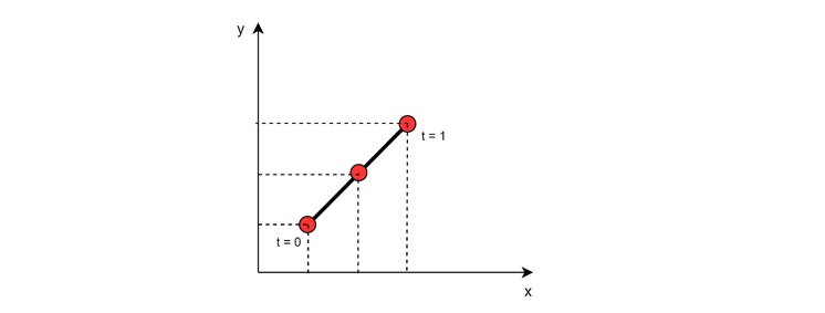
The idea behind linear interpolation is to find intermediate values between two endpoints. For that we use a parameter 't' that ranges from 0 to 1. When t = 0, we are at the start point. When t = 1, we are at the end point. Values of t between 0 and 1 give us points along the line connecting the start and end.

1D Linear Interpolation

For single dimensional case, the linear interpolation is the simplest form. It is used to find values between two numbers on a line.

For example, assume we have two numbers: 3 and 7. We want to find the halfway point between them.

• Start point (A) = 3
• End point (B) = 7
• t = 0.5 (halfway)

The formula is −

$$\mathrm{\text{Result} = (1 - t) \cdot A + t \cdot B}$$

Plugging in our values −

$$\mathrm{\text{Result} = (1 - 0.5) \cdot 3 + 0.5 \cdot 7 = 1.5 + 3.5 = 5}$$

So, the halfway point between 3 and 7 is 5.

2D Linear Interpolation

In 2D graphics, we often need to interpolate between two points in a plane. This is used to draw lines or create gradients.

The formula for 2D linear interpolation is −

$$\mathrm{p = (1 - t) a + t b}$$

Where,

• 'a' is the start point
• 'b' is the end point
• 't' is the interpolation parameter (0 to 1)
• 'p' is the resulting point

This formula creates a straight line between points 'a' and 'b'. As 't' varies from 0 to 1, 'p' moves along this line.

Linear Interpolation along the X-axis

A common use of linear interpolation in graphics is to create a continuous function from a set of discrete points. This is often done along the X-axis. Let's understand how it works ?.

We have a set of x-coordinates: x₀, x₁, ..., x_n. Each x-coordinate has an associated y-value: y₀, y₁, ..., y_n

We want to create a function f(x) that passes through all these points. Between any two adjacent points, we use linear interpolation. The formula for this type of interpolation is −

$$\mathrm{f(x) = y_i + \frac{(x - x_i)}{(x_{i+1} - x_i)} (y_{i+1} - y_i)}$$

Where,

• x_i and x_i+1 are two adjacent x-coordinates
• y_i and y_i+1 are their corresponding y-values
• x is any value between x_i and x_i+1

This formula creates straight line segments between each pair of adjacent points. It ensures that f(x_i) = y_i for all data points.

Applications of Linear Interpolation in Computer Graphics

Following are some of the important applications of Linear Interpolation in Computer Graphics −

• Drawing Lines − We have seen the mathematical details for linear interpolation. Let us see some examples. The linear interpolation is important for drawing lines on a screen. We use it to determine which pixels to color between two endpoints.
• Color Gradients − For color management and color gradients the interpolation technique is also used. We interpolate between two or more colors to create smooth transitions.
• Animation − We can see the effect of linear interpolation for smooth animation. It is used to calculate in-between frames for moving objects.
• Texture Mapping − Another possible use case is texture mapping on 3D objects. When applying textures to 3D models, linear interpolation helps map texture coordinates to screen coordinates.

Barycentric Coordinates

For more complex shapes like triangles, we use a special form of linear interpolation called barycentric coordinates.

Barycentric coordinates are a way to describe the location of a point in a triangle using three values. These values represent the influence of each vertex on the point. This works in the following way −

• Each vertex of the triangle is assigned a weight
• The weights always sum to 1
• Any point inside the triangle can be expressed as a weighted sum of the vertices

Barycentric coordinates are useful for interpolating values across a triangle. This is important for tasks like shading and texture mapping.

Conclusion

In this chapter, we explained the concept of linear interpolation in computer graphics. We started with the basic concept and formula. Then, we looked at how it works in different dimensions. We saw examples in 1D and 2D, and learned about interpolation along the X-axis.

We also discussed various applications of linear interpolation in graphics. These include drawing lines, creating color gradients, animation, and texture mapping. Finally, we introduced the concept of barycentric coordinates for triangle interpolation.