Solving Quadratic Equations in Computer Graphics

---

---

Quadratic equations are considered fundamental in algebra and they are used in many real-world applications. Quadratic equations form the basis for solving problems related to parabolic curves, projectile motion, and optimization. In this chapter, we will explain the basics of solving quadratic equations.

Quadratic Equations in Graphics

Before entering into the solving details, let us recap on what is the concept behind quadratic equation. These are the second-degree polynomial equation, generally expressed as −

$$\mathrm{Ax^2 + Bx + C = 0}$$

where,

• A, B, and C are constant coefficients,
• "x" is the variable we want to solve for.

For example, consider the following quadratic equation −

$$\mathrm{2x^2 + 6x + 4 = 0}$$

Here, A = 2, B = 6, and C = 4. The goal is to find the values of "x" that satisfy this equation.

Graphical Representation of Quadratic Equations

The graph of a quadratic equation forms a parabola. The shape of the parabola can vary based on the values of A, B, and C.

Note − If A > 0, the parabola opens upwards, and if A < 0, it opens downwards.

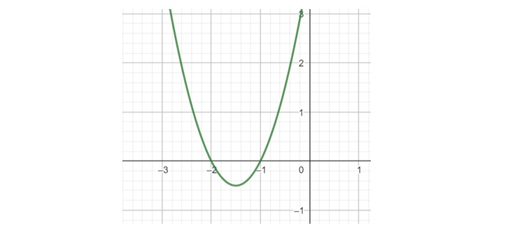
The x-intercepts (roots) of the parabola correspond to the values of x that make y = 0. In other words, these are the solutions to the quadratic equation.

A quadratic equation may have two solutions, one solution, or no real solution.

Quadratic Equation with Two Solutions

The parabola intersects the x-axis at two points.

Quadratic Solution with One Solution

In this case, the parabola just touches the x-axis (this is called a "double root").

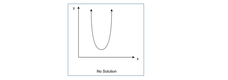
Quadratic Equation with No Real Solution

In this case, the parabola does not touch the x-axis, and the solutions are complex numbers.

Solving a Quadratic Equation

There are several methods to solve quadratic equations. We will explore the most common approaches: Factoring, Quadratic formula (Sridharacharya Acharyas Equation), and Completing the square.

Factoring

Factoring involves rewriting the quadratic equation as a product of two binomials. This method is simple but doesn't always work if the equation cannot be factored easily.

Example

$$\mathrm{\text{Solve }\: x^2 \:+\: 5x \:+\: 6 \:=\: 0}$$

We can factor the quadratic equation −

$$\mathrm{(x + 2)(x + 3) = 0}$$

Setting each factor to zero −

$$\mathrm{x + 2 = 0 \quad \text{or} \quad x + 3 = 0}$$

Thus, x = 2 or x = 3.

Quadratic Formula

When factoring is difficult or impossible, we use the quadratic formula (this is also known as Shreedhar Acharya's Formula), which works for any quadratic equation −

$$\mathrm{x = \frac{-B \pm \sqrt{B^2 - 4ac}}{2A}}$$

This formula directly gives us the solutions by plugging in the values of AAA, BBB, and CCC.

Example

Let us solve $\mathrm{2x^2 + 6x + 4 = 0}$ using the quadratic formula.

Here, A = 2, B = 6, and C = 4

Calculate the discriminant: $\mathrm{D = B^2 - 4AC}$

$$\mathrm{D = 6^2 - 4(2)(4) = 36 - 32 = 4}$$

Substitute into the quadratic formula −

$$\mathrm{x = \frac{-6 \pm \sqrt{4}}{2(2)} = \frac{-6 \pm 2}{4}}$$

Find the two solutions. The solutions are x = 1 and x = 2.

Completing the Square

Let us see the third method. To derive the quadratic formula or to solve certain types of quadratic equations using this method, it rewrites the quadratic equation in a perfect square form.

Following are the steps to complete the square −

• Start with the equation in the form $\mathrm{Ax^2 + Bx + C = 0}$ If $\mathrm{A \neq 1}$, divide the entire equation by $\mathrm{A}$.
• Move the constant term to the other side.
• Add the square of half the coefficient of $\mathrm{x}$ to both sides to create a perfect square trinomial on one side.
• Factor the trinomial and solve for $\mathrm{x}$.

Example

Solve $\mathrm{x^2 + 6x + 8 = 0}$ by completing the square.

Move the constant −

$$\mathrm{x^2 + 6x = -8}$$

Add $\mathrm{\left(\frac{6}{2}\right)^2 = 9}$ to both sides −

$$\mathrm{x^2 + 6x + 9 = 1}$$

Factor the left side −

$$\mathrm{(x + 3)^2 = 1}$$

Take the square root of both sides −

$$\mathrm{x + 3 = \pm 1}$$

Solve for x −

$$\mathrm{x = -3 + 1 = -2 \quad \text{or} \quad x = -3 - 1 = -4}$$

Discriminant and Nature of Roots

The discriminant D of a quadratic equation is the part of the quadratic formula under the square root −

$$\mathrm{D = B^2 - 4AC}$$

It helps us determine the nature of the solutions −

• If $\mathrm{D > 0}$, there are two real and distinct solutions.
• If $\mathrm{D = 0}$, there is one real and repeated solution (a double root).
• If $\mathrm{D < 0}$, there are two complex (imaginary) solutions.

Example

For the equation,

$$\mathrm{x^2 + x + 1 = 0}$$

Here, A = 1, B = 1, and C = 1

The discriminant is −

$$\mathrm{D = 12 - 4(1)(1) = 1 - 4 = -3}$$

Since $\mathrm{D < 0}$, the equation has two complex solutions.

Applications of Quadratic Equations

We have seen the methods, let us see the applications of Quadratic equations. These are particularly useful for solving problems involving projectile motion, optimization, and geometry and significant use in computer graphics for expressing curves.

• Modelling and processing quadric surfaces − A quadric equation can be defined by a homogeneous quadratic equation, where (x, y, z, w) are the homogeneous coordinates of a point in 3D space.
• Quadratic Bezier curves − A quadratic Bezier curve is defined by three control points, P0, P1, and P2. The points on a quadratic curve are defined as a linear interpolation of corresponding points on the linear Bezier curves from P0 to P1 and from P1 to P2.

Conclusion

In this chapter, we explained how to solve quadratic equations using different methods such as factoring, the quadratic formula, and completing the square. We also discussed the discriminant and how it determines the nature of the solutions. Lastly, we saw some applications of quadratic equations in real-world computer graphics domain.