Bias and Variance in Machine Learning

---

---

Bias and variance are two important concepts in machine learning that describe the sources of error in a model's predictions. Bias refers to the error that results from oversimplifying the underlying relationship between the input features and the output variable. At the same time, variance refers to the error that results from being too sensitive to fluctuations in the training data.

In machine learning, we strive to minimize both bias and variance in order to build a model that can accurately predict on unseen data. A high-bias model may be too simplistic and underfit the training data. In contrast, a model with high variance may overfit the training data and fail to generalize to new data.

Generally, a machine learning model shows three types of error - bias, variance, and irreducible error. There is a tradeoff between bias and variance errors. Decreasing the bias leads to increasing the variance and vice versa.

What is Bias?

Bias is calculated as the difference between average prediction and actual value. In machine learning, bias (systematic error) occurs when a model makes incorrect assumptions about data.

A model with high bias does not match well training data as well as test data. It leads to high errors in training and test data.

While the model with low bias matches the training data well (high training accuracy or less error in training). It leads to low error in training data but high error in test data.

Types of Bias

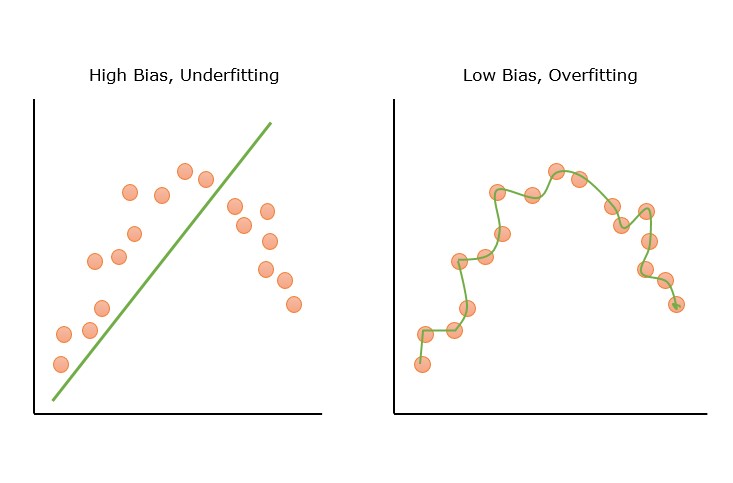
• High Bias − High bias occurs due to erroneous assumptions in the machine learning model. Models with high bias cannot capture the hidden pattern in the training data. This leads to underfitting.his leads to underfitting. Features of high bias are a highly simplified model, underfitting, and high error in training and test data.
• Low Bias − Models with low bias can capture the hidden pattern in the training data. Low bias leads to high variance and, eventually, overfitting. Low bias generally occurs due to the ML model being overly complex.

Below figure shows pictorial representation of the high and low bias error.

Example of Bias in Models

A linear regression model trying to fit the non-linear data will show a high bias. Some examples of models with high bias are linear regression and logistic regression. Some examples of models with low bias are decision trees, k-nearest neighbors, and support vector machines.

Impact of Bias on Model Performance

High bias can lead to poor performance on both training and test datasets. High-bias models will not be able to generalize on the new, unseen data.

What is Variance?

Variance is a measure of the spread or dispersion of numbers in a given set of observations with respect to the mean. It basically measures how a set of numbers is spread out from the average. In statistics and probability, variance is defined as the expectation of the squared deviation of a random variable from the sample mean.

In machine learning, variance is the variability of model prediction on different datasets. The variance shows how much model prediction varies when there is a slight variation in data. If model accuracies on training and test data vary greatly, the model has high variance.

A model with high variance can even fit noises on training data but lacks generalization to new, unseen data.

Types of Variance

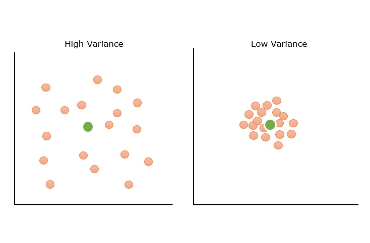
• High Variance − High variance models capture noise along with hidden pattern. It leads to overfitting. High variance models show high training accuracy but low test accuracy. Some features of a high variance model are an overly complex model, overfitting, low error on training data, and high error or test data.
• Low Variance − A model with low variance is unable to capture the hidden pattern in the data. Low variance may occur when we have a very small amount of data or use a very simplified model. Low variance leads to underfitting.

Below figure shows pictorial representation of the high and low variance examples.

Example of Variance in Models

A decision tree with many branches that fits the training data perfectly but does not fit properly on test data is an example of high variance. Examples of high variance: k-nearest neighbors, decision trees, and support vector machines (SVMs).

Impact of Variance on Model Performance

A high variance can lead to a model that performs well with training data but fails to perform well on training data. During training, high-variance models fit the training data so well that they even capture the noises as actual patterns. Models with high variance errors are known as overfitting models.

Bias-Variance Tradeoff

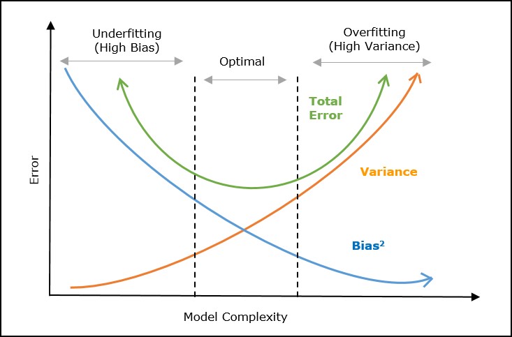
The bias-variance tradeoff is finding a balance between the error introduced by bias and the error introduced by variance. With increased model complexity, the bias will decrease, but the variance will increase. However, when we decrease the model complexity, the bias will increase, and the variance will decrease. So we need a balance between bias and variance so total prediction error is minimized.

A machine learning model will not perform well on new, unseen data if it has a high bias or variance in training. A good model should not have either high bias or variance. We can't reduce both bias and variance at the same time. When bias reduces, variance will increase. So we need to find an optimal bias and variance such that the prediction error is minimized.

In machine learning, bias-variance tradeoff is important because a model with high bias or high.

Graphical Representation

The following graph represents the tradeoff between bias and variance graphically.

In the above graph, the X-axis represents the model complexity, and the Y-axis represents the prediction error. The total error is the sum of bias error and variance error. The optimal region shows the area with the balance between bias and variance, showing optimal model complexity with minimum error.

Mathematical Representation

The prediction error in the machine learning model can be written mathematically as follows −

Error = bias² + variance + irreducible error.

To minimize the model prediction error, we need to choose model complexity in such a way so that a balance between these two errors can be met.

The main objective of the bias-variance tradeoff is to find optimal values of bias and variance (model complexity) that minimize the error.

Techniques to Balance Bias and Variance

There are different techniques to balance bias and variance to achieve an optimal prediction error.

1. Reducing High Bias

• Choosing a more complex model − As we have seen in the above diagram, choosing a more complex model may reduce the bias error of the model prediction.
• Adding more features − Adding mode features can increase the complexity of the model that can capture even better hidden patterns that will decrease the bias error of the model.
• Reducing regularization − Regularization prevents overfitting, but while decreasing the variance, it can increase bias. So, reducing the regularization parameters or removing regularization overall can reduce bias errors.

2. Reducing High Variance

• Applying regularization techniques − Regularization techniques add penalty to complex model that will eventually result in reduced complexity of the model. A less complex model will show less variance.
• Simplifying model complexity − A less complex model will have low variance. You can reduce the variance by using a simpler algorithm.
• Adding more data − Adding more data to the dataset can help the model to perform better showing less variance.
• Cross-validation − Cross-validation can be useful to identify overfitting by comparing the performance on training and validation sets of the datasets.

Bias and Variance Examples Using Python

Let's implement some practical examples using Python programming language. We have provided here four examples. The first three examples show some level of high/ low bias or variance. The fourth example shows the optimal value of both bias and variance.

Example of High Bias

Below is an implementation example in Python that illustrates how bias and variance can be analyzed using the Boston Housing dataset −

import numpy as np
import pandas as pd
from sklearn.datasets import load_boston

boston = load_boston()
X = boston.data
y = boston.target
from sklearn.model_selection import train_test_split

X_train, X_test, y_train, y_test = train_test_split(X, y, test_size=0.2,
random_state=42)
from sklearn.linear_model import LinearRegression
from sklearn.metrics import mean_squared_error

lr = LinearRegression()
lr.fit(X_train, y_train)

train_preds = lr.predict(X_train)
train_mse = mean_squared_error(y_train, train_preds)
print("Training MSE:", train_mse)

test_preds = lr.predict(X_test)
test_mse = mean_squared_error(y_test, test_preds)
print("Testing MSE:", test_mse)

Output

The output shows the training and testing mean squared errors (MSE) of the linear regression model. The training MSE is 21.64 and the testing MSE is 24.29, indicating that the model has a high level of bias and moderate variance.

Training MSE: 21.641412753226312
Testing MSE: 24.291119474973456

Example of Low Bias and High Variance

Let's try a polynomial regression model −

from sklearn.preprocessing import PolynomialFeatures

poly = PolynomialFeatures(degree=2)
X_train_poly = poly.fit_transform(X_train)
X_test_poly = poly.transform(X_test)

pr = LinearRegression()
pr.fit(X_train_poly, y_train)

train_preds = pr.predict(X_train_poly)
train_mse = mean_squared_error(y_train, train_preds)
print("Training MSE:", train_mse)

test_preds = pr.predict(X_test_poly)
test_mse = mean_squared_error(y_test, test_preds)
print("Testing MSE:", test_mse)

Output

The output shows the training and testing MSE of the polynomial regression model with degree=2. The training MSE is 5.31 and the testing MSE is 14.18, indicating that the model has a lower bias but higher variance compared to the linear regression model.

Training MSE: 5.31446956670908
Testing MSE: 14.183558207567042

Example of Low Variance

To reduce variance, we can use regularization techniques such as ridge regression or lasso regression. In the following example, we will be using ridge regression −

from sklearn.linear_model import Ridge

ridge = Ridge(alpha=1)
ridge.fit(X_train_poly, y_train)

train_preds = ridge.predict(X_train_poly)
train_mse = mean_squared_error(y_train, train_preds)
print("Training MSE:", train_mse)

test_preds = ridge.predict(X_test_poly)
test_mse = mean_squared_error(y_test, test_preds)
print("Testing MSE:", test_mse)

Output

The output shows the training and testing MSE of the ridge regression model with alpha=1. The training MSE is 9.03 and the testing MSE is 13.88 compared to the polynomial regression model, indicating that the model has a lower variance but slightly higher bias.

Training MSE: 9.03220937860839
Testing MSE: 13.882093755326755

Example of Optimal Bias and Variance

We can further tune the hyperparameter alpha to find the optimal balance between bias and variance. Let's see an example −

from sklearn.model_selection import GridSearchCV

param_grid = {'alpha': np.logspace(-3, 3, 7)}
ridge_cv = GridSearchCV(Ridge(), param_grid, cv=5)
ridge_cv.fit(X_train_poly, y_train)

train_preds = ridge_cv.predict(X_train_poly)
train_mse = mean_squared_error(y_train, train_preds)
print("Training MSE:", train_mse)

test_preds = ridge_cv.predict(X_test_poly)
test_mse = mean_squared_error(y_test, test_preds)
print("Testing MSE:", test_mse)

Output

The output shows the training and testing MSE of the ridge regression model with the optimal alpha value.

Training MSE: 8.326082686584716
Testing MSE: 12.873907256619141

The training MSE is 8.32 and the testing MSE is 12.87, indicating that the model has a good balance between bias and variance.