NumPy - Chi Square Distribution

---

---

What is the Chi-Square Distribution?

The Chi-Square Distribution is a continuous probability distribution used in statistics to test hypotheses about the variance of a population or the independence of two variables.

It is a special type of distribution derived from the sum of squares of independent standard normal random variables. Mathematically, if Z₁, Z₂, ..., Z_k are independent standard normal variables, then −

X = Z12 + Z22 + ... + Zk2

It is defined by the degrees of freedom (df), which depend on the number of independent variables in the dataset. This distribution is skewed and becomes more symmetric as the degrees of freedom increase.

Hence, the resulting variable, X, follows a Chi-Square distribution with k degrees of freedom. The degrees of freedom, denoted as k, play an important role in determining the shape of the distribution. Higher degrees of freedom result in a more symmetrical distribution.

Chi-Square Samples in NumPy

NumPy provides the numpy.random.chisquare() function to generate random samples from a Chi-Square distribution. This function requires two main parameters −

• df: Degrees of freedom.
• size (optional): The number of samples to generate.

Example: Generating Chi-Square Samples

The following example generates 10 random samples from a Chi-Square distribution with 5 degrees of freedom −

import numpy as np

# Generate Chi-Square samples
degrees_of_freedom = 5
samples = np.random.chisquare(degrees_of_freedom, size=10)
print("Generated Chi-Square samples:", samples)

Following is the output obtained −

Generated Chi-Square samples: [ 3.94124915  3.61732939  8.09217857  1.63322954  2.26579558  3.74957222
 10.88281092  1.98262239  3.816437   10.83575014]

Properties of the Chi-Square Distribution

The Chi-Square distribution has several important properties that make it useful for statistical analysis, they are −

• Asymmetry: The distribution is skewed to the right, especially for lower degrees of freedom. The skewness decreases as the degrees of freedom increase.
• Mean: The mean of the Chi-Square distribution is equal to its degrees of freedom (df).
• Variance: The variance is twice the degrees of freedom, or 2 * df.

Example

In the following example we are verifying mean and variance of the given degrees of freedom −

import numpy as np

# Verifying mean and variance
df = 5
samples = np.random.chisquare(df, size=1000)

mean = np.mean(samples)
variance = np.var(samples)

print("Mean of samples:", mean)
print("Variance of samples:", variance)

This will produce the following result −

Mean of samples: 5.04405316596172
Variance of samples: 10.565774002162097

Applications of the Chi-Square Distribution

The Chi-Square distribution is primarily used in hypothesis testing and variance estimation. Common applications are −

• Goodness-of-Fit Test: Evaluating how well a set of observed data matches a theoretical distribution.
• Test of Independence: Analyzing the independence of two categorical variables using a contingency table.
• Variance Analysis: Assessing the variability of a population or comparing variances of two populations.

Example: Goodness-of-Fit Test

Suppose we have observed frequencies of dice rolls and want to test whether the dice is fair using the Chi-Square distribution −

import numpy as np

# Observed and expected frequencies
observed = np.array([16, 18, 16, 14, 18, 18])
expected = np.array([15, 15, 15, 15, 15, 15])

# Chi-Square statistic
chi_square_stat = np.sum((observed - expected)**2 / expected)
print("Chi-Square statistic:", chi_square_stat)

This statistic can be compared to a critical value from the Chi-Square distribution table to determine the fairness of the dice −

Chi-Square statistic: 2.0

Visualizing the Chi-Square Distribution

Visualization helps in understanding the shape and characteristics of the Chi-Square distribution. We can use Matplotlib to plot its probability density function (PDF).

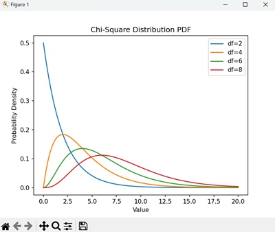
Example: Plotting the Chi-Square PDF

In the following example, we create a line plot showing the PDF of the Chi-Square distribution for varying degrees of freedom −

import numpy as np
import matplotlib.pyplot as plt
from scipy.stats import chi2

# Plotting PDF for different degrees of freedom
x = np.linspace(0, 20, 500)
dfs = [2, 4, 6, 8]

for df in dfs:
   plt.plot(x, chi2.pdf(x, df), label=f"df={df}")

plt.title("Chi-Square Distribution PDF")
plt.xlabel("Value")
plt.ylabel("Probability Density")
plt.legend()
plt.show()

The curves demonstrate how the distribution becomes less skewed as the degrees of freedom increase −

Simulating Real-World Scenarios

The Chi-Square distribution is often used in practical scenarios such as quality control and risk analysis. Let us simulate a real-world example of quality control in a manufacturing process.

Example: Quality Control in Manufacturing

Suppose a factory measures the variability of product dimensions. The Chi-Square distribution can test whether the variability is within acceptable limits. This statistic can be used to determine whether the observed variance exceeds the acceptable threshold −

import numpy as np

# Observed variance and acceptable threshold
observed_variance = 4.5
sample_size = 20
population_variance = 4.0

# Chi-Square statistic
chi_square_stat = (sample_size - 1) * observed_variance / population_variance
print("Chi-Square statistic:", chi_square_stat)

We get the output as shown below −

Chi-Square statistic: 21.375