NumPy - Zipf Distribution

---

---

What is the Zipf Distribution?

The Zipf Distribution is a discrete probability distribution that describes the frequency of elements ranked in descending order.

It follows the principle that the frequency of an element is inversely proportional to its rank in the frequency table, often seen in natural languages where the most common word appears twice as often as the second most common word, three times as often as the third, and so on.

It is defined by a parameter "s", which determines the skewness of the distribution. Example: The distribution of word frequencies in a large text corpus often follows a Zipf distribution. Mathematically, the probability mass function (PMF) of the Zipf distribution is given by:

P(X = k) = (1 / ks) / H(N, s)

Here, k is the rank, s is the exponent characterizing the distribution, and H(N, s) is the Nth generalized harmonic number, which normalizes the distribution.

Generating Zipf Samples in NumPy

NumPy provides the numpy.random.zipf() function to generate random samples from a Zipf distribution. This function requires two main parameters:

• a: The distribution parameter, also known as the exponent.
• size: The number of samples to generate (optional).

Example: Generating Zipf Samples

The following example generates 10 random samples from a Zipf distribution with an exponent of 2 −

import numpy as np

# Generate Zipf samples
a = 2
samples = np.random.zipf(a, size=10)
print("Generated Zipf samples:", samples)

Following is the output obtained −

Generated Zipf samples: [1 3 1 2 1 1 1 1 2 1]

Properties of the Zipf Distribution

The Zipf distribution has several unique properties that make it useful for modeling real-world phenomena, they are −

• Heavy Tail: The distribution has a heavy tail, meaning a small number of events are very common, while the majority are rare.
• Power Law: The probability of an event is inversely proportional to its rank raised to the power of the exponent.
• Scale-Invariant: The distribution remains the same when the scale of measurement changes.

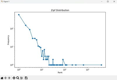
Example: Visualizing Zipf's Law

Let us visualize the Zipf distribution to understand its properties better. We can plot the frequency of occurrences of each rank using Matplotlib −

import numpy as np
import matplotlib.pyplot as plt

# Generate a large number of samples
a = 2
samples = np.random.zipf(a, size=1000)

# Count occurrences of each rank
unique, counts = np.unique(samples, return_counts=True)

# Plot the rank-frequency distribution
plt.figure(figsize=(10, 6))
plt.loglog(unique, counts, marker="o")
plt.title("Zipf Distribution")
plt.xlabel("Rank")
plt.ylabel("Frequency")
plt.show()

We obtained a log-log plot showing the frequency of each rank, demonstrating the heavy tail and power-law nature of the Zipf distribution −

Applications of the Zipf Distribution

The Zipf distribution is used in various fields to model phenomena where a few items are very common, and many items are rare. Common applications are −

• Natural Language Processing (NLP): Modeling word frequencies in a corpus.
• Population Studies: Analyzing city populations and sizes.
• Internet Traffic: Understanding the distribution of web page visits and hits.

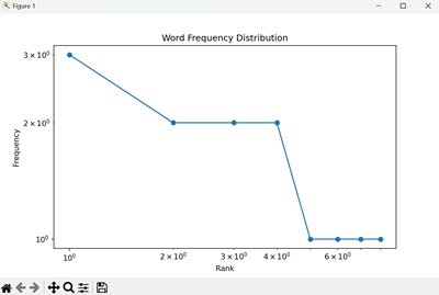
Example: Word Frequency in Text

Suppose we have a text document and want to model the frequency of words using the Zipf distribution −

import matplotlib.pyplot as plt
from collections import Counter

# Sample text
text = "the quick brown fox jumps over the lazy dog the quick brown fox"

# Split text into words
words = text.split()

# Count word frequencies
word_counts = Counter(words)

# Get ranks and frequencies
ranks = range(1, len(word_counts) + 1)
frequencies = [count for word, count in word_counts.most_common()]

# Plot the rank-frequency distribution
plt.figure(figsize=(10, 6))
plt.loglog(ranks, frequencies, marker="o")
plt.title("Word Frequency Distribution")
plt.xlabel("Rank")
plt.ylabel("Frequency")
plt.show()

We obtain a log-log plot showing the frequency of each word rank in the text, following the Zipf distribution −

Estimating Zipf's Exponent

In real-world applications, we often need to estimate the exponent parameter of the Zipf distribution. This can be done using various statistical techniques. One simple method is to fit a line to the log-log plot of rank vs. frequency.

Example: Estimating the Exponent

In the example below, the estimated exponent is close to the actual value (a = 2), demonstrating the accuracy of the estimation method −

import numpy as np
from scipy.stats import linregress

# Generate a large number of samples
a = 2
samples = np.random.zipf(a, size=1000)

# Count occurrences of each rank
unique, counts = np.unique(samples, return_counts=True)

# Perform linear regression on the log-log plot
log_ranks = np.log(unique)
log_counts = np.log(counts)
slope, intercept, r_value, p_value, std_err = linregress(log_ranks, log_counts)

print("Estimated exponent:", -slope)

The output obtained is as shown below −

Estimated exponent: 0.8852106553815038

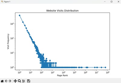
Simulating Real-World Scenarios

Let us simulate a real-world scenario using the Zipf distribution. Suppose we want to model the distribution of website visits on a popular news site.

Example: Website Visits

We can generate a large number of samples from a Zipf distribution and analyze the distribution of visits to different pages −

import matplotlib.pyplot as plt
import numpy as np

# Generate Zipf samples
a = 1.5
samples = np.random.zipf(a, size=10000)

# Count occurrences of each page visit
unique, counts = np.unique(samples, return_counts=True)

# Plot the rank-frequency distribution
plt.figure(figsize=(10, 6))
plt.loglog(unique, counts, marker="o")
plt.title("Website Visits Distribution")
plt.xlabel("Page Rank")
plt.ylabel("Visit Frequency")
plt.show()

We obtain a log-log plot showing the distribution of website visits, demonstrating the heavy tail and power-law nature of the Zipf distribution −