SciPy - Linear 1-D Interpolation

---

---

SciPy Linear 1-D Interpolation is a method used to estimate unknown values between two known data points in one dimension by assuming a linear relationship between adjacent points. This is useful when we have discrete data and want to create a smooth function that approximates intermediate values. In SciPy the interp1d() function from the scipy.interpolate module is used to perform this interpolation.

Linear interpolation works by connecting two points with a straight line and then calculating any intermediate points along that line. This approach is computationally efficient but assumes a constant rate of change between data points which may not be accurate for more complex data.

Working of Linear Interpolation

Linear interpolation works by estimating the value of a function between two known points by assuming that the function behaves linearly between those points. The given two known data points are (x₀,y₀) and (x₁,y₁) and now the linear interpolation finds an estimated value as y at a point x between x₀ and x₁.

The formula to calculate the interpolated value y for a given x is given as follows −

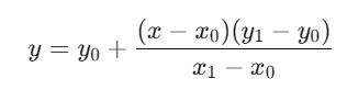
Where, (x₀,y₀) and (x₁,y₁) are the known data points, x is the point where we want to estimate the value and y is the interpolated value.

Linear interpolation assumes a straight-line relationship between adjacent points by making it simple and efficient but not suitable for data with nonlinear patterns.

For example if we have known data points as (1,3) and (4,7) then we can estimate the value at x = 2, the linear interpolation would be computed as 4.33.

Syntax

Following is the syntax of generating the 1-d interpolation in scipy with the help of scipy.interpolate.inter1d() function −

scipy.interpolate.interp1d(x, y, kind='linear', axis=-1, copy=True, bounds_error=None, fill_value=np.nan, assume_sorted=False)

Parameters

Here are the parameters of the scipy.interpolate.inter1d() function −

• x: Array of independent data points.
• y: Array of dependent data points. It should have the same length as x.
• kind: This parameters specifies the type of interpolation to perform. Common options are 'linear'(default) which is linear interpolation between points and 'nearest', 'zero', 'slinear', 'quadratic', 'cubic' are for different kinds of interpolation.
• axis: This parameter specifies the axis of y along which to interpolate and the default value is -1 for the last axis.
• copy: If True then the arrays x and y are copied. Default value is True.
• bounds_error: If True then an error is raised if a value outside the range of x is requested. Default value is None which uses fill_value instead.
• fill_value: Value to return for x values outside the interpolation range. Default value is np.nan.
• assume_sorted: If True then the input arrays are assumed to be sorted. Default value is False.

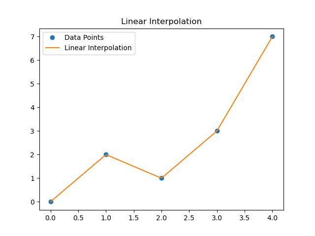
Linear Interpolation

Here is the example of the generating the linear interpolation with the use of scipy.interpolate.inter which connects the data points with straight lines.

import numpy as np
import matplotlib.pyplot as plt
from scipy.interpolate import interp1d

# Known data points
x = np.array([0, 1, 2, 3, 4])
y = np.array([0, 2, 1, 3, 7])

# Linear interpolation
f_linear = interp1d(x, y, kind='linear')

# Interpolated points
x_new = np.linspace(0, 4, 100)
y_new = f_linear(x_new)

# Plotting
plt.plot(x, y, 'o', label='Data Points')
plt.plot(x_new, y_new, '-', label='Linear Interpolation')
plt.legend()
plt.title('Linear Interpolation')
plt.show()

Below is the output of the linear 1-D interpolation in scipy −

Cubic Interpolation

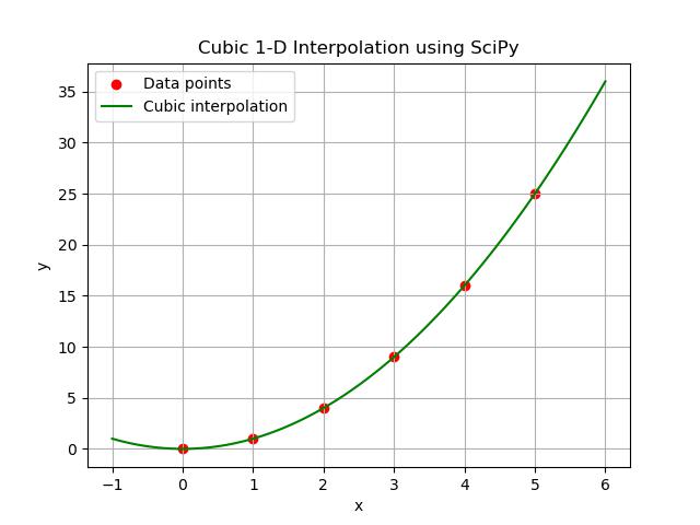
Cubic interpolation is a more advanced interpolation method compared to linear interpolation. It fits a cubic polynomial between data points by resulting in a smoother curve that better captures the behavior of nonlinear data. This method is useful when we need smoother transitions between points as it avoids the sharp changes that can occur with linear interpolation.

SciPy provides cubic interpolation through the interp1d() function in the scipy.interpolate module by specifying the parameter as kind='cubic'.

Here is the example of generating the cubic interpolation using the scipy.interpolate.inter1d() function by passing the parameter kind = 'cubic' −

import numpy as np
import matplotlib.pyplot as plt
from scipy.interpolate import interp1d

# Known data points (nonlinear function)
x = np.array([0, 1, 2, 3, 4, 5])
y = np.array([0, 1, 4, 9, 16, 25])

# Create a cubic interpolation function
cubic_interp = interp1d(x, y, kind='cubic', fill_value='extrapolate')

# Generate new x values for interpolation
x_new = np.linspace(-1, 6, 100)

# Interpolate the y values at the new x values
y_new = cubic_interp(x_new)

# Plot the original data points
plt.scatter(x, y, color='red', label='Data points')

# Plot the cubic interpolation
plt.plot(x_new, y_new, label='Cubic interpolation', color='green')

# Adding labels and legend
plt.title('Cubic 1-D Interpolation using SciPy')
plt.xlabel('x')
plt.ylabel('y')
plt.legend()
plt.grid(True)

# Display the plot
plt.show()

Here is the output of the Cubic 1-D interpolation in scipy library using the inter1d() function −

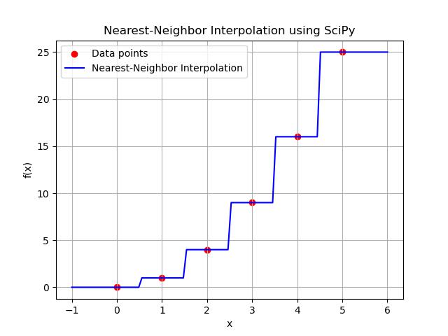
Nearest-Neighbor Interpolation

Nearest-neighbor interpolation is the simplest form of interpolation where the value of an unknown point is assigned to the value of the nearest known data point. This method does not attempt to create a smooth curve or continuous transitions between data points instead it selects the value of the closest available point by making it fast and computationally inexpensive.

In SciPy the nearest-neighbor interpolation can be performed using the interp1d function from the scipy.interpolate module by setting the kind parameter to 'nearest'.

Here is the example of generating the Nearest-Neighbor Interpolation using the scipy.interpolate.inter1d() function by passing the parameter kind = 'nearest' −

import numpy as np
import matplotlib.pyplot as plt
from scipy.interpolate import interp1d

# Known data points
x = np.array([0, 1, 2, 3, 4, 5])
y = np.array([0, 1, 4, 9, 16, 25])

# Create a nearest-neighbor interpolation function
nearest_interp = interp1d(x, y, kind='nearest', fill_value='extrapolate')

# Generate new x values for interpolation
x_new = np.linspace(-1, 6, 100)

# Interpolate the y values at the new x values
y_new = nearest_interp(x_new)

# Plot the original data points
plt.scatter(x, y, color='red', label='Data points')

# Plot the nearest-neighbor interpolation
plt.plot(x_new, y_new, label='Nearest-Neighbor Interpolation', color='blue')

# Adding labels and legend
plt.title('Nearest-Neighbor Interpolation using SciPy')
plt.xlabel('x')
plt.ylabel('f(x)')
plt.legend()
plt.grid(True)

# Display the plot
plt.show()

Following is the output of the Nearest Neighbour 1-D interpolation in scipy library using the inter1d() function −

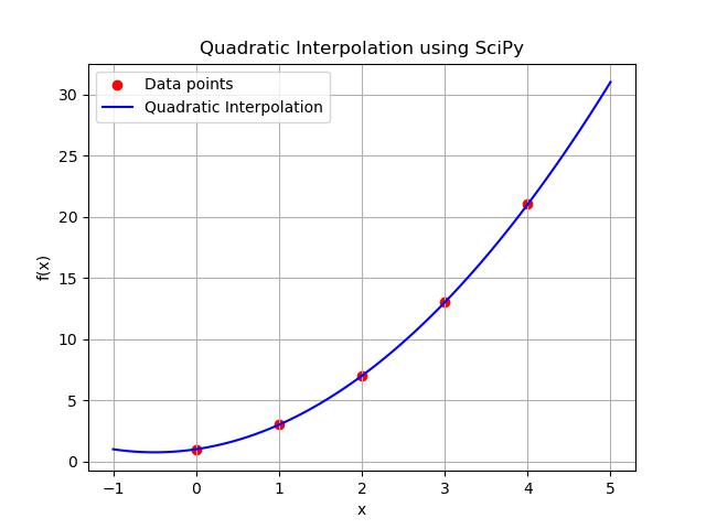
Quadratic Interpolation

Quadratic interpolation is a method that fits a quadratic function i.e., a second-degree polynomial to three or more data points by allowing for a smooth curve to approximate the data. It is more accurate than linear interpolation because it captures curvature but it is less complex and computationally demanding than higher-order interpolation methods such as cubic interpolation.

In SciPy quadratic interpolation can be performed using the interp1d() function from the scipy.interpolate module by setting the kind parameter to quadratics.

Following is the example of generating the Quadratic 1d Interpolation using the scipy.interpolate.inter1d() function by passing the parameter kind = 'quadratic' −

import numpy as np
import matplotlib.pyplot as plt
from scipy.interpolate import interp1d

# Known data points
x = np.array([0, 1, 2, 3, 4])
y = np.array([1, 3, 7, 13, 21])

# Create a quadratic interpolation function
quadratic_interp = interp1d(x, y, kind='quadratic', fill_value='extrapolate')

# Generate new x values for interpolation
x_new = np.linspace(-1, 5, 100)

# Interpolate the y values at the new x values
y_new = quadratic_interp(x_new)

# Plot the original data points
plt.scatter(x, y, color='red', label='Data points')

# Plot the quadratic interpolation
plt.plot(x_new, y_new, label='Quadratic Interpolation', color='blue')

# Adding labels and legend
plt.title('Quadratic Interpolation using SciPy')
plt.xlabel('x')
plt.ylabel('f(x)')
plt.legend()
plt.grid(True)

# Display the plot
plt.show()

Below is the output of the Quadratic 1-D interpolation in scipy library using the inter1d() function −

Benefits of Linear 1-D Interpolation

Here are the benefits of using the Linear 1-D Interpolation in scipy −

• Simple and Efficient: Linear interpolation is computationally inexpensive and straightforward to implement.
• Approximation: It provides a reasonable estimate when data points follow a near-linear trend.

Limitations of Linear 1-D Interpolation

We can see some limitations of using the Linear 1-D Interpolation in Scipy −

• Accuracy: Linear interpolation may not be suitable for data with significant non-linearity as it doesn't capture curves or changes in gradient.
• Sharp Corners: The piecewise linear approach can introduce discontinuities in the derivative of the interpolated function.