SciPy - Bilateral Filter

---

---

A Bilateral Filter is a nonlinear, edge-preserving and noise-reducing smoothing filter. It smooths images while preserving edges by weighting pixel values with a spatial Gaussian filter and an intensity Gaussian filter.

SciPy does not have a built-in bilateral filter but it can be implemented using the scipy.ndimage module or other libraries like OpenCV.

Key Features of Bilateral Filter

Following are the key features of the Bilateral Filter which is used in SciPy Image Processing −

• Edge Preservation: The Bilateral filter is designed to preserve edges while reducing noise. It smooths regions that are spatially close and have similar intensity values while keeping sharp edges intact. This makes it especially useful for tasks where edge information is critical such as in image denoising and pre-processing for segmentation.
• Non-Linear Filtering: Unlike linear filters such as Gaussian filters, the bilateral filter is non-linear because it combines both the spatial distance and intensity difference between neighboring pixels to compute a weighted average. This non-linearity helps to preserve the edges of objects in the image.
• Dual Gaussian Filters: The bilateral filter uses two Gaussian functions namely, Spatial Gaussian which determines the spatial distance i.e., the Euclidean distance between pixels to decide how much influence neighboring pixels have and Intensity Guassian which considers the intensity i.e., color or grayscale difference between neighboring pixels to determine how much influence a pixel will have based on its similarity to the center pixel.
• Edge-Aware Smoothing: This filter performs smoothing by adjusting the weight of each pixel based not only on its spatial distance but also its intensity difference from the target pixel. This makes it ideal for applications where we want to reduce noise while preserving the edges as the filter will not smooth across edges with high intensity differences.
• Parameter Sensitivity: There are two methods namely, sigma spatial(_spatial) which is used to how much spatial distance influences the filter. Larger values means that pixels farther from the center pixel will have a higher weight and sigma Intensity(_Intensity) which controls how much the intensity difference influences the filter. Larger values reduce the edge-preserving effect and increase smoothing even across intensity differences.
• Local Adaptive Filtering: The Bilateral filter adapts to the local features of the image. It adjusts the amount of filtering applied based on both the pixels spatial location and its intensity similarity to neighboring pixels. This leads to a more context-sensitive result compared to traditional linear filters.
• Computational Complexity: The Bilateral filter is computationally expensive because it requires the calculation of pixel similarity for each pixel in a neighborhood by making it slower than linear filters. The complexity increases with the size of the filter kernel and the image.
• Noise Reduction: Bilateral filters are especially effective at reducing various types of noise such as Gaussian noise or salt-and-pepper noise without blurring the edges of objects in the image.

Advantages of Bilateral Filter

Here are the advantages of the Scipy Bilateral Filter used in Image processing −

• Edge Preservation: The traditional filters that smooth across edges where the bilateral filter keeps edges sharp.
• Noise Removal: This filter is effective in removing various types of noise especially in high-resolution images.
• Local Adaptability: The filter adapts to local image features by considering both spatial proximity and intensity similarity.

Disadvantages of Bilateral Filter

Bilateral Filter have the advantages as well as the disadvantages which can be defined as follows −

• Computationally Intensive: In the Bilateral Filter the need of computing the intensity and spatial weights for each pixel makes the bilateral filter slower than other traditional smoothing filters, especially for large images.
• Parameter Tuning: In this filter the parameter tuning for choosing appropriate values for the spatial and intensity sigma values can be tricky and requires experimentation for different images.

Implementing a Bilateral Filter in SciPy

Implementing a bilateral filter in SciPy requires combining spatial and intensity domain Gaussian weighting to smooth images while preserving edges.

SciPy itself does not have a direct bilateral filter implementation but we can create one using its utilities such as scipy.ndimage.gaussian_filter() and NumPy for computations.

Syntax

Following is the syntax of the scipy.ndimage.gaussian_filter() function which can be used to apply the Bilateral filter in scipy −

scipy.ndimage.gaussian_filter(
   input, 
   sigma, 
   order=0, 
   output=None, 
   mode='reflect', 
   cval=0.0, 
   truncate=4.0
)

Here are the parameters of the function scipy.ndimage.gaussian_filter() −

• input: The input array such as an image as a NumPy array.
• sigma: Standard deviation for the Gaussian kernel. It can be a single number or a sequence for each axis.
• order: This is the derivative order where 0 for a regular Gaussian blur and higher values compute derivatives.
• output(optional): This is the output array to store the result.
• mode: This parameter determines how the array borders are handled and the modes are such as reflect, constant, nearest, mirror and wrap.
• cval: This is the constant value to fill edges if mode='constant'.
• truncate: This parameter is used to truncate the filter at this many standard deviations.

Example

Following is the example of implementing the Bilateral filter using the scipy.ndimage.guassian_filter() function of scipy −

import numpy as np
from scipy.ndimage import gaussian_filter
from skimage import data
import matplotlib.pyplot as plt
 
# load an image
image = data.camera()
sigma_s = 5
sigma_r = 20
def bilateral_filter(image, sigma_s, sigma_r):
   # Ensure the image is a floating-point array
   image = image.astype(np.float64)
   
   # Create a grid of spatial coordinates
   radius = int(3 * sigma_s)  # Typically, 3*sigma_s is used as the filter radius
   y, x = np.mgrid[-radius:radius+1, -radius:radius+1]
   
   # Spatial Gaussian weights
   spatial_gaussian = np.exp(-(x**2 + y**2) / (2 * sigma_s**2))
   
   # Initialize the output image
   output = np.zeros_like(image)
   normalizer = np.zeros_like(image)
   
   # Iterate over each pixel
   for i in range(radius, image.shape[0] - radius):
      for j in range(radius, image.shape[1] - radius):
         # Extract the local patch
         patch = image[i-radius:i+radius+1, j-radius:j+radius+1]
         
         # Compute the intensity Gaussian weights
         intensity_gaussian = np.exp(-((patch - image[i, j])**2) / (2 * sigma_r**2))
         
         # Combine the spatial and intensity weights
         weights = spatial_gaussian * intensity_gaussian
         
         # Normalize weights
         weights /= weights.sum()
         
         # Compute the filtered pixel value
         output[i, j] = np.sum(patch * weights)
         normalizer[i, j] = weights.sum()
   
   return output
    
bilateral_image  = bilateral_filter(image, sigma_s, sigma_r)
# Display original and Filtered images
plt.figure(figsize=(12, 6))
plt.subplot(1, 2, 1)
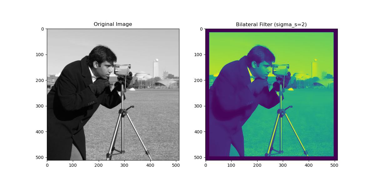
plt.title("Original Image")
plt.imshow(image, cmap="gray")

plt.subplot(1, 2, 2)
plt.title("Bilateral Filter (sigma_s=2)")
plt.imshow(bilateral_image)
plt.show()

Here is the output of the Bilateral filter with the help of scipy.ndimage.guassian_filter() function −

Implementing Bilateral Filter using OpenCV

OpenCV provides a highly optimized implementation of bilateral filtering through the cv2.bilateralFilter() function. This function is much faster than a custom implementation and is well-suited for real-time applications.

Here is the example of implementing the Bilateral Filtering through the cv2.bilateralFilter() function in OpenCV −

import cv2
import matplotlib.pyplot as plt

# Load a color image
image = cv2.imread("\images\images.jpeg") 
# Check if the image was loaded correctly
if image is None:
    print("Error: Unable to load image. Check the file path.")
else:
   # Convert from BGR to RGB (OpenCV loads images in BGR by default)
   image = cv2.cvtColor(image, cv2.COLOR_BGR2RGB)
   
   # Apply bilateral filter
   filtered_image = cv2.bilateralFilter(image, d=15, sigmaColor=80, sigmaSpace=80)
   
   # Display the original and filtered images
   plt.figure(figsize=(12, 6))
   plt.subplot(1, 2, 1)
   plt.title("Original Image")
   plt.imshow(image)
   plt.axis('off')
   
   plt.subplot(1, 2, 2)
   plt.title("Bilateral Filtered Image")
   plt.imshow(filtered_image)
   plt.axis('off')
   
   plt.show()

Following is the output of the Bilateral Function through OpenCV −