SciPy - Continuous Wavelet Transform (CWT)

---

---

Continuous Wavelet Transform in SciPy

The Continuous Wavelet Transform (CWT) is a powerful signal processing technique used to analyze signals in both the time and frequency domains simultaneously. Unlike the, Fourier Transform which provides global frequency content, CWT allows for multi-resolution analysis by making it particularly useful for signals with time-varying frequency content (non-stationary signals).

The Continuous Wavelet Transform of a signal x(t) is defined by the following integral −

W(a, b) = - x(t) * ( (t - b) / a ) dt

Where −

• x(t) is the input signal.
• (t) is the mother wavelet and a function localized in both time and frequency.
• ^* is the complex conjugate of the wavelet function.
• is the scale parameter i.e.,controls the dilation or compression of the wavelet, related to frequency.
• b is the translation parameter i.e., controls the shifting in time.
• W(a,b) represents the wavelet coefficients that provide a measure of similarity between the signal and the wavelet at different scales and time positions.

Key Properties of CWT

Following are the key properties of the Continuous Wavelet Transform −

• Time-Frequency Localization: CWT provides information about when and at what frequency a particular event occurs.
• Multi-Resolution Analysis: Small scales (low a) capture high-frequency details i.e., sharp features and Large scales (high a) capture low-frequency components i.e., smooth variations.
• Redundancy: CWT is highly redundant compared to Discrete Wavelet Transform (DWT) by making it computationally expensive but useful for detailed analysis.

Note:

In SciPy versions 1.15.1 and later the cwt function has been removed from the scipy.signal module. Therefore, if you're using SciPy 1.15.1 or higher, we should use alternative methods to perform the Continuous Wavelet Transform (CWT) such as the PyWavelets (pywt) library.

Using PyWavelets (pywt)

If We're facing issues with SciPy's cwt function, an alternative approach is to use PyWavelets (pywt), a powerful library for wavelet analysis in Python. It provides extensive functionality for Continuous Wavelet Transform (CWT), Discrete Wavelet Transform (DWT) and more.

Installing PyWavelets

To install PyWavelets in our working environment we have to run the following command in the command prompt −

pip install pywavelets

Following is the output after executing the above command −

Successfully installed pywavelets-1.8.0

Verifying the installation with the help of below command −

import pywt
print(pywt.__version__)

Following is the output of the installed version of PyWavelets −

1.8.0

Basic Example of CWT using PyWavelets

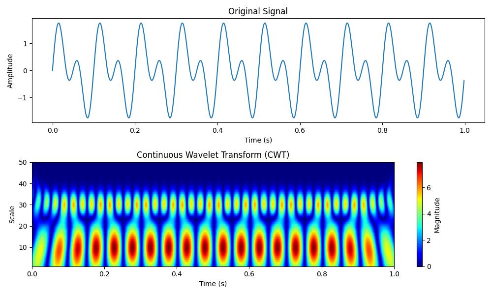
Following is a basic example of performing a Continuous Wavelet Transform (CWT) using the PyWavelets (pywt) library. This example analyzes a simple signal using the Morlet wavelet which is commonly used for time-frequency analysis −

import numpy as np
import pywt
import matplotlib.pyplot as plt

# Generate a simple signal: combination of two sine waves (10 Hz and 20 Hz)
t = np.linspace(0, 1, 500, endpoint=False)  # Time vector (1 second, 500 samples)
signal = np.sin(2 * np.pi * 10 * t) + np.sin(2 * np.pi * 20 * t)  # Signal

# Define the range of scales for wavelet transform
scales = np.arange(1, 50)

# Perform Continuous Wavelet Transform using the Morlet wavelet
coefficients, frequencies = pywt.cwt(signal, scales, 'morl')

# Plot the original signal
plt.figure(figsize=(10, 6))
plt.subplot(2, 1, 1)
plt.plot(t, signal)
plt.title("Original Signal")
plt.xlabel("Time (s)")
plt.ylabel("Amplitude")

# Plot the CWT coefficients as a heatmap
plt.subplot(2, 1, 2)
plt.imshow(np.abs(coefficients), extent=[0, 1, 1, 50], cmap='jet', aspect='auto',
           vmax=abs(coefficients).max(), vmin=0)
plt.colorbar(label="Magnitude")
plt.title("Continuous Wavelet Transform (CWT)")
plt.xlabel("Time (s)")
plt.ylabel("Scale")
plt.tight_layout()
plt.show()

Following is the output of the Continuous Wavelet Transform using PyWavelets −

Detecting a Transient Event (Gaussian Pulse)

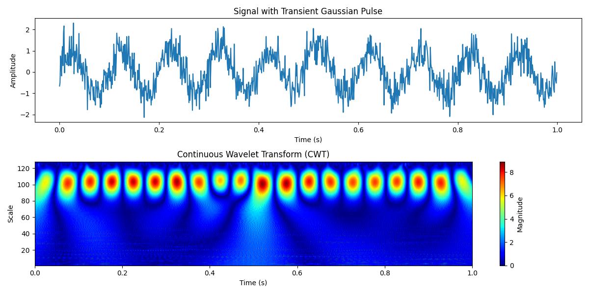
In this example we will see how to use PyWavelets to detect a transient event such as a Gaussian pulse, within a time series signal. The Continuous Wavelet Transform (CWT) can help identify the presence and timing of such transient events −

import numpy as np
import pywt
import matplotlib.pyplot as plt

# Generate a time vector
t = np.linspace(0, 1, 1000, endpoint=False)  # 1 second, 1000 samples

# Create a signal with a Gaussian pulse embedded in noise
signal = np.sin(2 * np.pi * 10 * t)  # Background sine wave (10 Hz)
gaussian_pulse = np.exp(-((t - 0.5)**2) / (2 * 0.01**2))  # Gaussian pulse at t = 0.5s
noise = np.random.normal(0, 0.5, t.shape)  # Random noise

# Final signal (sine wave + transient pulse + noise)
signal += gaussian_pulse + noise

# Define wavelet scales for analysis
scales = np.arange(1, 128)

# Perform Continuous Wavelet Transform using the Ricker (Mexican Hat) wavelet
coefficients, frequencies = pywt.cwt(signal, scales, 'mexh')

# Plot the original signal
plt.figure(figsize=(12, 6))
plt.subplot(2, 1, 1)
plt.plot(t, signal)
plt.title("Signal with Transient Gaussian Pulse")
plt.xlabel("Time (s)")
plt.ylabel("Amplitude")

# Plot the CWT coefficients as a heatmap
plt.subplot(2, 1, 2)
plt.imshow(np.abs(coefficients), extent=[0, 1, 1, 128], cmap='jet', aspect='auto',
           vmax=abs(coefficients).max(), vmin=0)
plt.colorbar(label="Magnitude")
plt.title("Continuous Wavelet Transform (CWT)")
plt.xlabel("Time (s)")
plt.ylabel("Scale")
plt.tight_layout()
plt.show()

Following is the output of the Detecting Transient event by using the CWT in PyWavelets −

Choosing the Right Wavelet

Choosing the right wavelet for performing Continuous Wavelet Transform (CWT) depends on the specific characteristics of the signal we're analyzing and the type of features we want to capture. Different wavelets have different properties that make them more suitable for certain types of signals. Heres a guide to help we choose the right wavelet −

Wavelet	Best For	Example Use Cases
Ricker (Mexican Hat)	Transient pulses, sharp features	Detecting spikes, Gaussian pulses
Morlet	Oscillatory signals, time-frequency analysis	EEG, audio signals, periodic signals
Gaussian	Smooth, non-oscillatory signals	Gradual transitions, denoising
Haar	Discontinuous signals, edge detection	Signal compression, sharp transitions
Morse	Time-frequency analysis of broad signals	Seismic, bio-signals (EEG, ECG), multiresolution analysis