- SciPy - Home
- SciPy - Introduction
- SciPy - Environment Setup
- SciPy - Basic Functionality
- SciPy - Relationship with NumPy
- SciPy Clusters
- SciPy - Clusters
- SciPy - Hierarchical Clustering
- SciPy - K-means Clustering
- SciPy - Distance Metrics
- SciPy Constants
- SciPy - Constants
- SciPy - Mathematical Constants
- SciPy - Physical Constants
- SciPy - Unit Conversion
- SciPy - Astronomical Constants
- SciPy - Fourier Transforms
- SciPy - FFTpack
- SciPy - Discrete Fourier Transform (DFT)
- SciPy - Fast Fourier Transform (FFT)
- SciPy Integration Equations
- SciPy - Integrate Module
- SciPy - Single Integration
- SciPy - Double Integration
- SciPy - Triple Integration
- SciPy - Multiple Integration
- SciPy Differential Equations
- SciPy - Differential Equations
- SciPy - Integration of Stochastic Differential Equations
- SciPy - Integration of Ordinary Differential Equations
- SciPy - Discontinuous Functions
- SciPy - Oscillatory Functions
- SciPy - Partial Differential Equations
- SciPy Interpolation
- SciPy - Interpolate
- SciPy - Linear 1-D Interpolation
- SciPy - Polynomial 1-D Interpolation
- SciPy - Spline 1-D Interpolation
- SciPy - Grid Data Multi-Dimensional Interpolation
- SciPy - RBF Multi-Dimensional Interpolation
- SciPy - Polynomial & Spline Interpolation
- SciPy Curve Fitting
- SciPy - Curve Fitting
- SciPy - Linear Curve Fitting
- SciPy - Non-Linear Curve Fitting
- SciPy - Input & Output
- SciPy - Input & Output
- SciPy - Reading & Writing Files
- SciPy - Working with Different File Formats
- SciPy - Efficient Data Storage with HDF5
- SciPy - Data Serialization
- SciPy Linear Algebra
- SciPy - Linalg
- SciPy - Matrix Creation & Basic Operations
- SciPy - Matrix LU Decomposition
- SciPy - Matrix QU Decomposition
- SciPy - Singular Value Decomposition
- SciPy - Cholesky Decomposition
- SciPy - Solving Linear Systems
- SciPy - Eigenvalues & Eigenvectors
- SciPy Image Processing
- SciPy - Ndimage
- SciPy - Reading & Writing Images
- SciPy - Image Transformation
- SciPy - Filtering & Edge Detection
- SciPy - Top Hat Filters
- SciPy - Morphological Filters
- SciPy - Low Pass Filters
- SciPy - High Pass Filters
- SciPy - Bilateral Filter
- SciPy - Median Filter
- SciPy - Non - Linear Filters in Image Processing
- SciPy - High Boost Filter
- SciPy - Laplacian Filter
- SciPy - Morphological Operations
- SciPy - Image Segmentation
- SciPy - Thresholding in Image Segmentation
- SciPy - Region-Based Segmentation
- SciPy - Connected Component Labeling
- SciPy Optimize
- SciPy - Optimize
- SciPy - Special Matrices & Functions
- SciPy - Unconstrained Optimization
- SciPy - Constrained Optimization
- SciPy - Matrix Norms
- SciPy - Sparse Matrix
- SciPy - Frobenius Norm
- SciPy - Spectral Norm
- SciPy Condition Numbers
- SciPy - Condition Numbers
- SciPy - Linear Least Squares
- SciPy - Non-Linear Least Squares
- SciPy - Finding Roots of Scalar Functions
- SciPy - Finding Roots of Multivariate Functions
- SciPy - Signal Processing
- SciPy - Signal Filtering & Smoothing
- SciPy - Short-Time Fourier Transform
- SciPy - Wavelet Transform
- SciPy - Continuous Wavelet Transform
- SciPy - Discrete Wavelet Transform
- SciPy - Wavelet Packet Transform
- SciPy - Multi-Resolution Analysis
- SciPy - Stationary Wavelet Transform
- SciPy - Statistical Functions
- SciPy - Stats
- SciPy - Descriptive Statistics
- SciPy - Continuous Probability Distributions
- SciPy - Discrete Probability Distributions
- SciPy - Statistical Tests & Inference
- SciPy - Generating Random Samples
- SciPy - Kaplan-Meier Estimator Survival Analysis
- SciPy - Cox Proportional Hazards Model Survival Analysis
- SciPy Spatial Data
- SciPy - Spatial
- SciPy - Special Functions
- SciPy - Special Package
- SciPy Advanced Topics
- SciPy - CSGraph
- SciPy - ODR
- SciPy Useful Resources
- SciPy - Reference
- SciPy - Quick Guide
- SciPy - Cheatsheet
- SciPy - Useful Resources
- SciPy - Discussion
SciPy - Curve Fitting
Curve fitting is the process of constructing a mathematical function that best approximates a set of data points. In SciPy the curve_fit() function from the scipy.optimize module is commonly used to fit a given model which typically nonlinear to the data. The goal is to find the optimal parameters of the model that minimize the differences i.e. residuals between the data and the model's predicted values.
How Curve Fitting Works?
As we know Curve fitting is the process of finding a curve that best describes the relationship between a set of data points. In detail, heres how it works −
- Data Points: The data consists of independent variable(s) and dependent variable . These points represent observations or measurements.
- Model Selection: Choose a mathematical model such as linear, polynomial, exponential that represents the underlying trend. The model has parameters that need to be determined to fit the data.
- Objective: The objective is to find the parameters of the model such that the curve minimizes the difference i.e. error between the predicted values model() and the observed data .
-
Error Calculation: The error can be calculated using a loss function which is typically the sum of squared errors (SSE) given as follows −
SSE = (observed - model)2
This ensures that larger differences contribute more heavily to the total error.
- Optimization: An optimization technique such as least squares is applied to adjust the model parameters to minimize the error.
- Curve Fitting Tools: SciPys curve_fit() function is widely used. It takes the model function, data and an initial guess for the parameters and returns the optimal parameters that fit the data.
Types of Curve fittings
There are several types of curve fitting techniques depending on the nature of the data and the model used. These can range from simple linear fits to more complex nonlinear models. Here are the main types of curve fitting used in SciPy −
| Type of Curve Fitting | Definition | Model Equation | Use Case |
|---|---|---|---|
| Linear | A method that fits a straight line to data points, showing a constant rate of change between variables. | y = ax + b | When the relationship is approximately linear. |
| Polynomial | A method that uses a polynomial equation to fit data points, capturing more complex relationships. | y = an xn + an-1 xn-1 + ... + a0 | For smooth, nonlinear relationships (e.g., quadratic, cubic). |
| Exponential | A fitting method used when data exhibits exponential growth or decay, commonly seen in natural phenomena. | y = a ebx + c | Data that grows or decays exponentially. |
| Logarithmic | A fitting method that models relationships where the rate of change decreases over time. | y = a log(x) + b | When growth slows down as the independent variable increases. |
| Power Law | A method that models data where one variable changes as a power of another variable, often in scale-invariant phenomena. | y = axb | When a variable changes as a power of another variable. |
| Sigmoidal (Logistic) | A method that fits an S-shaped curve, commonly used for growth processes that saturate. | y = a / (1 + e-b(x - c)) | For S-shaped curves in growth or saturation models. |
| Gaussian | A fitting method that models data with a bell-shaped distribution, typical in statistical analyses. | y = a e-(x - b)2 / (2c2) | For bell-shaped data distributions (normal distribution). |
| Rational Function | A method that fits a ratio of polynomial equations to describe more complex relationships between variables. | y = (an xn + ... + a0) / (bm xm + ... + b0) | For more complex relationships that require ratios of polynomials. |
Understanding the Results
Understanding the results of curve fitting involves interpreting the output from the fitting process and evaluating how well the model describes the data.
- Fitted Parameters: The estimated parameters minimize the difference between the actual data and the predicted values of the model function.
- Covariance Matrix: The covariance matrix gives insights into the accuracy of the parameter estimates. Diagonal elements represent the variance of each parameter by helping us understand the confidence in the fitted values.
Curve Fitting vs Interpolation
Curve fitting focuses on modeling the relationship between variables for predictive purposes while interpolation is concerned with estimating values between known data points by ensuring precision within the observed range. The choice between the two techniques depends on the goals of the analysis and the nature of the data.
Here's a comparison of curve fitting and interpolation −
| Aspect | Curve Fitting | Interpolation |
|---|---|---|
| Definition | Finds a curve that best represents the relationship between data points. | Estimates values between known data points. |
| Purpose | Models underlying trends for predictions and insights. | Provides precise estimates within the known range. |
| Methods | Least squares fitting, polynomial fitting, regression analysis. | Linear interpolation, polynomial interpolation, spline interpolation. |
| Mathematical Approach | Minimizes error between the fitted curve and data points. | Constructs new points ensuring the function passes through known data. |
| Applicability | Used for understanding relationships and generalization (e.g., regression). | Used for precise value estimation (e.g., numerical methods). |
| Extrapolation | Allows extrapolation beyond the observed data range, but with caution. | Does not involve extrapolation but estimates are only within known data range. |
| Output | A smooth curve that may not pass through all data points. | A curve that passes exactly through all known data points. |
SciPy Function for Curve Fitting
We have the function scipy.optimize.curve_fit() to perform the curve fitting in scipy.
| S.No | Function & Description |
|---|---|
| 1 |
scipy.optimize.curve_fit() Fits a function to data using non-linear least squares. Allows users to define custom models for fitting and returns the optimal parameters that best describe the data. |
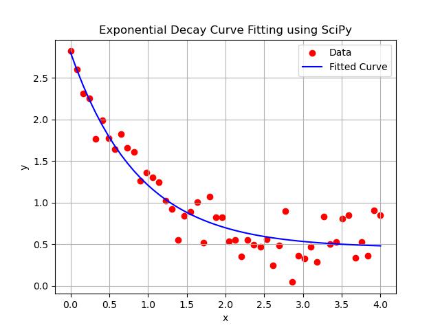
Following is the example which demonstrates how to fit an exponential decay function to data using curve_fit() function −
import numpy as np
import matplotlib.pyplot as plt
from scipy.optimize import curve_fit

# Define the model function (exponential decay)
def model_func(x, a, b, c):
    return a * np.exp(-b * x) + c

# Generate synthetic data (noisy exponential decay)
x_data = np.linspace(0, 4, 50)
y_data = model_func(x_data, 2.5, 1.3, 0.5) + np.random.normal(0, 0.2, size=x_data.shape)

# Perform curve fitting
# Initial guess for parameters a, b, c is optional but can speed up convergence
params, params_covariance = curve_fit(model_func, x_data, y_data, p0=[2, 1, 0])

# Generate data from the fitted curve
y_fitted = model_func(x_data, *params)

# Plot original noisy data and the fitted curve
plt.scatter(x_data, y_data, label='Data', color='red')
plt.plot(x_data, y_fitted, label='Fitted Curve', color='blue')

# Add labels and title
plt.title('Exponential Decay Curve Fitting using SciPy')
plt.xlabel('x')
plt.ylabel('y')
plt.legend()
plt.grid(True)
plt.show()

# Print the fitted parameters
print(f"Fitted parameters: a = {params[0]}, b = {params[1]}, c = {params[2]}")
Following is the output of curve fitting in scipy −