SciPy - Discontinuous Functions

---

---

What are Discontinuous Functions?

A Discontinuous function is a type of mathematical function that does not have a well-defined limit at certain points in its domain which means that at least one point in the functions domain leads to a sudden jump or break in its value.

In the view of numerical analysis and scientific computing with libraries such as SciPy, handling discontinuous functions is important for accurate calculations especially in integration and optimization tasks.

Characteristics of Discontinuous Functions

Discontinuous functions in SciPy exhibit several key characteristics that can complicate numerical computations especially integration.

Understanding these characteristics is crucial for effectively integrating and working with discontinuous functions in SciPy. Here are the features of the Discontinuous Functions −

• Abrupt Changes: Discontinuous functions have sudden jumps or breaks in value at specific points by making them non-smooth. This can lead to difficulties in defining their integrals.
• Undefined Behavior: At points of discontinuity this function may be undefined or infinite which can result in integration errors or warnings.
• Non-differentiability: Discontinuous functions are typically not differentiable at their points of discontinuity which affect methods that rely on derivative calculations.
• Piecewise Definition: Many discontinuous functions are defined piece wise with different expressions for different intervals. Handling these requires careful setup in integration routines.
• Integration Challenges: Traditional numerical integration methods may struggle with discontinuous functions which requires adaptive techniques or interval splitting to achieve accurate results.
• Oscillation Around Discontinuities: In some cases a discontinuous function may oscillate near its discontinuities by complicating the integration further due to rapid changes in value.
• Special Handling Required: Functions with known discontinuities often need special treatment such as using quad() with specified integration limits or splitting the intervals to avoid integrating across the discontinuity.
• Sensitivity to Tolerance Settings: The numerical results can be sensitive to the error tolerance parameters such as epsabs, epsrel which set in integration functions with necessary adjustments for accuracy.

Handling Discontinuous Functions in SciPy

When dealing with discontinuous functions in SciPy it's important to ensure accurate integration and other numerical methods. Here are the important steps how to handle them effectively −

• Identifying Discontinuities: Identifying points of discontinuity is essential. This can be done by analyzing the function mathematically or graphically. If the discontinuities are known beforehand they can be incorporated into numerical methods.

• Integration with SciPy: The scipy.integrate module provides several tools for integrating functions which includes those with discontinuities. The key function for integration is quad() which can handle a variety of cases including discontinuities.

  When we use the points parameter in the quad() function then the points argument can specify known points of discontinuity by allowing the integrator to adjust its calculations accordingly.

  If the function has multiple discontinuities then we can integrate the function in segments to avoid regions where the function is not continuous.

• Optimization with SciPy: When optimizing functions with discontinuities then the SciPy optimization module can be used but care must be taken. Some optimization algorithms might struggle with discontinuities so using methods like minimize_scalar with appropriate bounds is advisable.

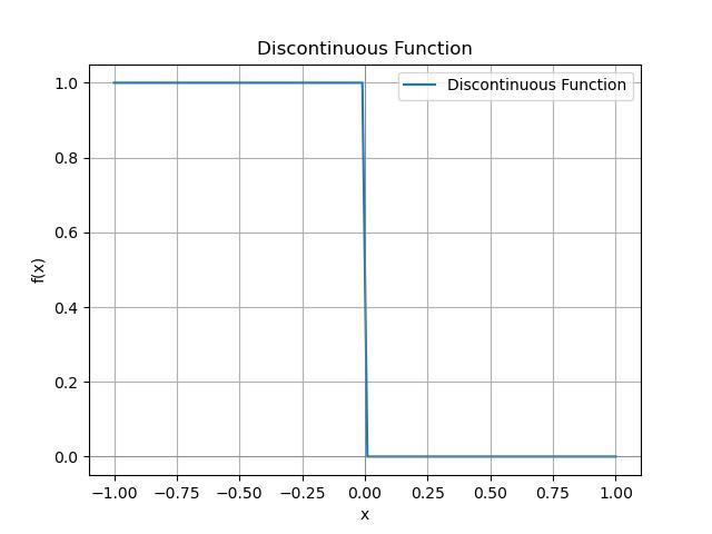
Simple Discontinuous Function

Following is the example of the simple Discontinuous Function −

import numpy as np
import matplotlib.pyplot as plt
from scipy.integrate import quad

# Define a discontinuous function
def discontinuous_function(x):
    return 1 if x < 0 else 0

# Plot the function
x = np.linspace(-1, 1, 100)
y = [discontinuous_function(val) for val in x]

plt.plot(x, y, label='Discontinuous Function')
plt.axhline(0, color='grey', lw=0.5)
plt.axvline(0, color='grey', lw=0.5)
plt.title("Discontinuous Function")
plt.xlabel("x")
plt.ylabel("f(x)")
plt.legend()
plt.grid()
plt.show()

# Integrate the function
integral1, error1 = quad(discontinuous_function, -1, 0)
integral2, error2 = quad(discontinuous_function, 0, 1)
total_integral = integral1 + integral2
print(f"Integral from -1 to 0: {integral1}, Integral from 0 to 1: {integral2}, Total Integral: {total_integral}")

Here is the output of the simple Discontinuous Function in scipy −

Different Discontinuous Functions

Following are the different types of discontinuous functions that we can use in numerical analysis and each with unique properties that can affect calculations and integrations in SciPy −

Function Name	Description
Step Function	This function jumps from one value to another at a specific point. It is often used to model sudden changes.
Piecewise Function	Defined differently over different intervals with leading to discontinuities at transition points. Common in mathematical modeling.
Dirichlet Function	This function is 1 at rational numbers and 0 at irrational numbers by making it highly discontinuous across its domain.
Heaviside Step Function	A variation of the step function used in control systems. It is 0 for negative inputs and 1 for positive inputs.
Sine Function with Jump	A modified sine function that introduces a jump at a specific point by demonstrating discontinuity in periodic functions.
Removable Discontinuity	This function is not defined at a specific point but can be defined to make it continuous. It illustrates the concept of removable discontinuity.

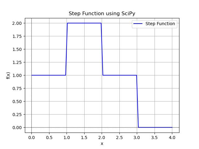
Step function

A step function is a piecewise constant function that takes constant values on intervals and has discontinuities at certain points where it jumps from one value to another. This behavior makes it useful for modeling systems that experience sudden changes or transitions. We can use the step function with the help of scipy.interpolate module.

Following are the characteristics of the step function −

• Constant Value: This function remains constant within specified intervals.
• Discontinuity: This function jump discontinuities at the points where it changes value.
• Common Applications: Step functions are often used in control systems, signal processing and mathematical modeling to represent thresholds or on/off conditions.

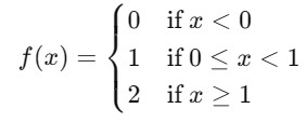
The Mathematical Representation of the simple Step function can be given as follows −

Example

In this example we will define a step function that takes on different constant values in specified intervals −

 
import numpy as np
import matplotlib.pyplot as plt
from scipy.interpolate import interp1d

# Define the step function data points
x_points = [0, 1, 2, 3]
y_points = [1, 2, 1, 0]  # The function values at the step points

# Create a step function using scipy.interpolate
step_function = interp1d(x_points, y_points, kind='previous', fill_value='extrapolate')

# Generate x values for plotting
x_values = np.linspace(-1, 4, 100)
y_values = step_function(x_values)

# Plotting the step function
plt.plot(x_values, y_values, label='Step Function', color='blue')
plt.title('Step Function using SciPy')
plt.xlabel('x')
plt.ylabel('f(x)')
plt.axhline(0, color='black', lw=0.5, ls='--')
plt.axvline(0, color='black', lw=0.5, ls='--')
plt.grid()
plt.legend()
plt.show()

Following is the output of the step function created in scipy −

Piecewise Function

A piecewise function is defined by multiple sub-functions with each applying to a certain interval of the input variable. These functions may have different rules in different intervals which leads to discontinuities at the boundaries between intervals.

Characteristics of the piecewise function are given as follows −

• Multiple Definitions: The function can take different forms based on the input interval.
• Discontinuity: It may exhibit discontinuities at the points where the definition changes.
• Applications: Used in various mathematical modeling scenarios including economics and engineering.

The Mathematical Representation of a piecewise function can be given as follows −

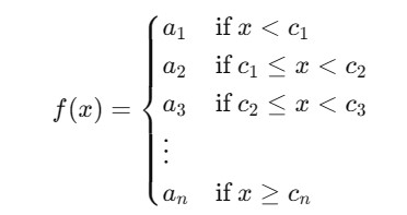
Example

In this example, we will define a piecewise function with different expressions based on intervals using SciPy −

import numpy as np
import matplotlib.pyplot as plt
from scipy.interpolate import interp1d

# Define the piecewise function data points
x_points = [-2, 0, 1, 3]  # Interval boundaries
y_points = [0, 1, 0, -1]  # Function values at the specified points

# Create a piecewise function using scipy.interpolate
piecewise_function = interp1d(x_points, y_points, kind='linear', fill_value='extrapolate')

# Generate x values for plotting
x_values = np.linspace(-3, 4, 100)
y_values = piecewise_function(x_values)

# Plotting the piecewise function
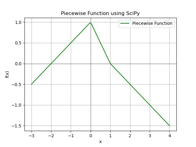
plt.plot(x_values, y_values, label='Piecewise Function', color='green')
plt.title('Piecewise Function using SciPy')
plt.xlabel('x')
plt.ylabel('f(x)')
plt.axhline(0, color='black', lw=0.5, ls='--')
plt.axvline(0, color='black', lw=0.5, ls='--')
plt.grid()
plt.legend()
plt.show()

Following is the output of the piecewise function created in SciPy −

Dirichlet Function

The Dirichlet function is defined to be 1 at rational numbers and 0 at irrational numbers. This function is not Riemann integrable by making it an interesting example in analysis.

Characteristics of the Dirichlet function are given as follows −

• Rational vs Irrational: It takes the value 1 at rational points and 0 at irrational points.
• Discontinuity: It is discontinuous everywhere in its domain.
• Mathematical Interest: Often discussed in real analysis and measure theory.

Let () be a function defined on a domain . The Dirichlet boundary condition specifies that the function takes on prescribed values on the boundary of the domain. This can be expressed mathematically as follows −

()= () for   

Where, ()is the function whose behavior is being studied within the domain , () is a known function that specifies the values that must take on the boundary and is the boundary of the domain where the Dirichlet condition is applied.

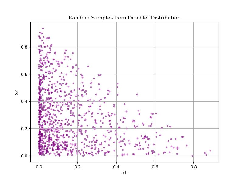
Example

In this example we will show how the Dirichlet function is used in SciPy −

import numpy as np
import matplotlib.pyplot as plt
from scipy.stats import dirichlet

# Define alpha parameters (concentration parameters)
alpha = [0.5, 1.0, 2.0]

# Generate a random sample from the Dirichlet distribution
sample = dirichlet.rvs(alpha, size=1000)

# Plot the sample data for visualization
plt.figure(figsize=(8, 6))

# Plot 2D projection of the Dirichlet samples (first 2 components)
plt.scatter(sample[:, 0], sample[:, 1], s=10, color='purple', alpha=0.5)
plt.title('Random Samples from Dirichlet Distribution')
plt.xlabel('x1')
plt.ylabel('x2')

plt.grid(True)
plt.show()

Following is the output of the Dirichlet function created in SciPy −

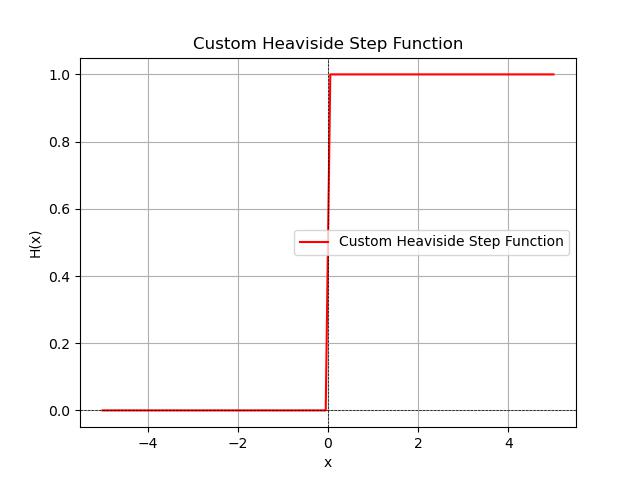
Heaviside Step Function

The Heaviside step function is a discontinuous function used in mathematics and engineering to represent the effect of turning on or off a switch. It is defined as 0 for negative inputs and 1 for non-negative inputs.

Following are the characteristics of the Heaviside step function −

• Switching Behavior: Represents the switch being off for negative inputs and on for non-negative inputs.
• Discontinuity: Has a jump discontinuity at zero.
• Applications: Used extensively in control systems and signal processing.

The Mathematical Representation of the Heaviside function can be given as follows −

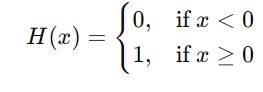
Example

In this example, we will define the Heaviside step function using SciPy −

import numpy as np
import matplotlib.pyplot as plt

# Define a custom Heaviside step function
def heaviside(x):
    return np.where(x < 0, 0, 1)

# Define the x values
x_values = np.linspace(-5, 5, 100)

# Apply the custom Heaviside step function to the x values
y_values = heaviside(x_values)

# Plotting the Heaviside step function
plt.plot(x_values, y_values, label='Custom Heaviside Step Function', color='red')
plt.title('Custom Heaviside Step Function')
plt.xlabel('x')
plt.ylabel('H(x)')
plt.axhline(0, color='black', lw=0.5, ls='--')
plt.axvline(0, color='black', lw=0.5, ls='--')
plt.grid(True)
plt.legend()
plt.show()

Here is the output of the Heaviside function created in SciPy −

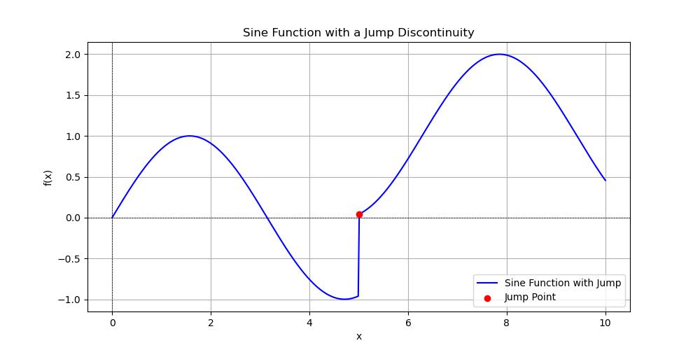
Sine Function with Jump

A sine function with a jump is a modified version of the sine function that experiences a sudden shift in value at a certain point. This function combines oscillatory behavior with discontinuity.

Below are the characteristics of the sine function with a jump −

• Oscillation: Exhibits periodic oscillations like the standard sine function.
• Jump Discontinuity: Contains a sudden increase or decrease at a specified point.
• Applications: Useful in modeling situations where a sudden change occurs in an otherwise periodic behavior.

The mathematical representation of a sine function with a jump can be expressed as a piecewise function. For example consider a sine function that has a jump discontinuity at a certain point say at = . Then the piecewise function can be defined as follows −

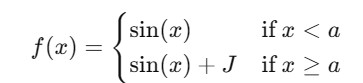
Here represents the magnitude of the jump at = .

Example

In this example we will define a sine function with a jump discontinuity using SciPy library −

import numpy as np
import matplotlib.pyplot as plt
from scipy.interpolate import interp1d

# Define the x values
x = np.linspace(0, 10, 500)

# Define the sine function with a jump at x=5
y = np.sin(x)
y[x > 5] += 1  # Create a jump in the function at x=5

# Create a piecewise function for better handling of the jump
x_points = [0, 5, 10]  # Points where the function changes
y_points = [np.sin(0), np.sin(5), np.sin(10) + 1]  # Corresponding function values

# Create an interpolation function
piecewise_func = interp1d(x_points, y_points, fill_value="extrapolate")

# Generate y values for the piecewise function
y_piecewise = piecewise_func(x)

# Plotting
plt.figure(figsize=(10, 5))
plt.plot(x, y, label='Sine Function with Jump', color='blue')
plt.scatter(5, np.sin(5) + 1, color='red', label='Jump Point', zorder=5)  # Marking the jump
plt.title('Sine Function with a Jump Discontinuity')
plt.xlabel('x')
plt.ylabel('f(x)')
plt.axhline(0, color='black', lw=0.5, ls='--')
plt.axvline(0, color='black', lw=0.5, ls='--')
plt.grid(True)
plt.legend()
plt.show()

Following is the output of the sine function with a jump created in SciPy −

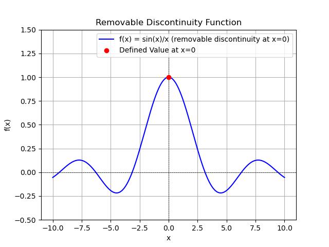
Removable Discontinuity

A removable discontinuity occurs in a function when it is not defined at a certain point, but it could be defined in such a way that the limit exists at that point. This makes it possible to "remove" the discontinuity by redefining the function at that point.

Characteristics of removable discontinuity −

• Undefined Point: The function is not defined at the discontinuous point.
• Limit Exists: The limit of the function approaches a finite value as the input approaches the discontinuous point.
• Applications: Useful in calculus and analysis for illustrating concepts of limits and continuity.

The Mathematical Representation of a removable discontinuity can be given as follows −

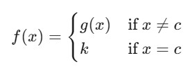
Where, g(x) is a function that is continuous at = and k is defined such that = lim().

Example

In this example we will define a function with a removable discontinuity using scipy.interp1d module −

import numpy as np
import matplotlib.pyplot as plt
from scipy.interpolate import interp1d

# Define the piecewise function
def piecewise_function(x):
    return np.where(x != 0, np.sin(x) / x, 1)  # sin(x)/x for x != 0, and 1 at x=0

# Generate x values
x_values = np.linspace(-10, 10, 1000)
y_values = piecewise_function(x_values)

# Plotting the function
plt.plot(x_values, y_values, label='f(x) = sin(x)/x (removable discontinuity at x=0)', color='blue')

# Highlight the discontinuity
plt.scatter([0], [1], color='red', label='Defined Value at x=0', zorder=5)
plt.axhline(0, color='black', lw=0.5, ls='--')
plt.axvline(0, color='black', lw=0.5, ls='--')

# Set plot limits and labels
plt.ylim(-0.5, 1.5)
plt.title('Removable Discontinuity Function')
plt.xlabel('x')
plt.ylabel('f(x)')
plt.grid()
plt.legend()
plt.show()

Following is the output of the function with removable discontinuity created in SciPy −