Scipy Discrete Fourier Transform (DFT)

---

---

Discrete Fourier Transform

The Discrete Fourier Transform (DFT) in SciPy is a numerical method for converting a sequence of time-domain data points into its frequency-domain representation. It reveals the amplitude and phase of different frequency components in a signal.

SciPy implements DFT through the scipy.fft module which provides efficient computation using the Fast Fourier Transform (FFT) algorithm by reducing computation time significantly.

It includes functions such as fft and ifft for 1D signals and fft2, ifft2 for 2D signals. DFT is commonly used in signal processing, image analysis and audio analysis to analyze frequency characteristics and filter signals.

The Mathematical formula to calculate the Discrete Fourier Transform(DFT) of a sequence x[n] of length N is given as follows −

Where −

• X[k] represents the DFT of [] at frequency index k.
• x[n] is the original time-domain signal at index n.
• The exponential value is complex exponential representing the basis functions of different frequencies.
• j is the imaginary value = 0, 1, 2,...., N-1.

Frequency Bins

The DFT transforms the signal into N frequency bins in which each bin representing a discrete frequency component of the original signal. The index k corresponds to a frequency of k/N times of the sampling rate. For real-valued signals the DFT output exhibits symmetry with the first half representing positive frequencies and the second half negative frequencies.

Magnitude and Phase

In the Discrete Fourier Transform (DFT) magnitude and phase are key aspects used to describe the frequency content of a signal. Let's see them in detail −

Magnitude in DFT

The magnitude indicates the strength or amplitude of each frequency present in the signal. If the DFT of a signal x[n] is represented as X[k], where X[k] is a complex number then the magnitude is given as follows −

where, Re(X[k]) and Im(X[k]) represent the real and imaginary parts respectively. The magnitude shows how much energy is concentrated at each frequency.

Phase in DFT

The phase provides information about the timing or horizontal shift of each frequency component. The phase of X[k] is determined as follows −

The phase describes how the frequency components align in time and for real signals, the phase tends to be symmetric.

Significance of Magnitude and Phase

The significance of magnitude and phase are given as follows −

• The magnitude helps understand the intensity of different frequencies in the signal.
• The phase shows the alignment of each frequency component in time.

Both components magnitude and phase are essential for a full understanding of the signals frequency content. When using the inverse DFT (IDFT) to reconstruct the time-domain signal both magnitude and phase are required for accurate signal recovery.

Example

Here's an example which shows how to compute and visualize the magnitude and phase of a signal using the Discrete Fourier Transform (DFT) with Python and SciPy −

import numpy as np
import matplotlib.pyplot as plt
from scipy.fft import fft, fftfreq

# Create a sample signal
sampling_rate = 1000  # Sampling rate in Hz
T = 1.0 / sampling_rate  # Sampling interval
t = np.linspace(0.0, 1.0, sampling_rate, endpoint=False)  # Time vector
# Create a signal with two frequencies: 50 Hz and 120 Hz
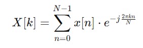
signal = 0.5 * np.sin(2.0 * np.pi * 50.0 * t) + 0.3 * np.sin(2.0 * np.pi * 120.0 * t)

# Compute the DFT of the signal
X = fft(signal)
N = len(signal)  # Number of sample points
frequencies = fftfreq(N, T)[:N//2]  # Positive frequencies

# Compute the magnitude and phase
magnitude = np.abs(X)[:N//2]  # Magnitude of DFT
phase = np.angle(X)[:N//2]    # Phase of DFT

# Plot the signal
plt.figure(figsize=(14, 6))
plt.subplot(2, 1, 1)
plt.plot(t, signal)
plt.title("Time-Domain Signal")
plt.xlabel("Time (s)")
plt.ylabel("Amplitude")

# Plot the magnitude spectrum
plt.subplot(2, 1, 2)
plt.plot(frequencies, magnitude)
plt.title("Magnitude Spectrum")
plt.xlabel("Frequency (Hz)")
plt.ylabel("Magnitude")
plt.grid()

# Show the plots
plt.tight_layout()
plt.show()

# Print phase information
for freq, ph in zip(frequencies, phase):
    print(f"Frequency: {freq:.2f} Hz, Phase: {ph:.2f} radians")

Following is the output of the Magnitude and Phase of the Discrete Fourier Transform(DFT) −

Frequency: 0.00 Hz, Phase: -3.14 radians
Frequency: 1.00 Hz, Phase: -1.08 radians
Frequency: 2.00 Hz, Phase: -1.85 radians
Frequency: 3.00 Hz, Phase: -0.19 radians
Frequency: 4.00 Hz, Phase: 1.18 radians
----------------------------------------
----------------------------------------
----------------------------------------
Frequency: 496.00 Hz, Phase: -0.43 radians
Frequency: 497.00 Hz, Phase: -2.43 radians
Frequency: 498.00 Hz, Phase: -0.15 radians
Frequency: 499.00 Hz, Phase: 2.54 radians

Applications of DFT

The Discrete Fourier Transform (DFT) is widely used in various fields for analyzing the frequency components of discrete signals. Below are the common applications of DFT −

• Signal Processing: DFT helps in analyzing the frequency content of signals by enabling tasks such as filtering, noise reduction and modulation.
• Audio Analysis: DFT is used in applications such as speech recognition, music analysis and audio compression by breaking down audio signals into their frequency components.
• Image Processing: DFT is applied to images for tasks such as image filtering, compression and reconstruction especially for frequency domain analysis.
• Communications: In digital communications DFT is used in OFDM systems for efficient data transmission and channel estimation.
• Spectral Analysis: The DFT is used for analyzing the power spectrum of signals to identify periodicities and detect patterns in data.

These applications increase the ability of DFT to transform time-domain data into the frequency domain by providing valuable insights into the signal's characteristics.

Example

Below is the example of calculating the Discrete Fourier Transform in Scipy −

import numpy as np
import matplotlib.pyplot as plt

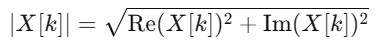
# Sample signal: A combination of two sine waves (5 Hz and 20 Hz)
sampling_rate = 100  # samples per second
T = 1.0 / sampling_rate  # sample spacing
t = np.linspace(0.0, 1.0, sampling_rate, endpoint=False)  # time vector
signal = np.sin(2.0 * np.pi * 5.0 * t) + 0.5 * np.sin(2.0 * np.pi * 20.0 * t)

# Compute the DFT of the signal
N = len(signal)  # number of sample points
dft = np.fft.fft(signal)
frequencies = np.fft.fftfreq(N, T)

# Take only the positive half of the DFT (as it is symmetric)
positive_frequencies = frequencies[:N//2]
magnitude = np.abs(dft[:N//2])

# Plot the time-domain signal
plt.figure(figsize=(12, 6))
plt.subplot(2, 1, 1)
plt.plot(t, signal)
plt.title("Time-Domain Signal")
plt.xlabel("Time [s]")
plt.ylabel("Amplitude")

# Plot the magnitude of the DFT (Frequency-Domain Signal)
plt.subplot(2, 1, 2)
plt.stem(positive_frequencies, magnitude, basefmt=" ")
plt.title("Magnitude Spectrum (DFT)")
plt.xlabel("Frequency [Hz]")
plt.ylabel("Magnitude")
plt.grid()

# Show plots
plt.tight_layout()
plt.show()

Following is the output of the calculating the Discrete Fourier Transform(DFT) in Scipy −

Inverse Discrete Fast Fourier Transform

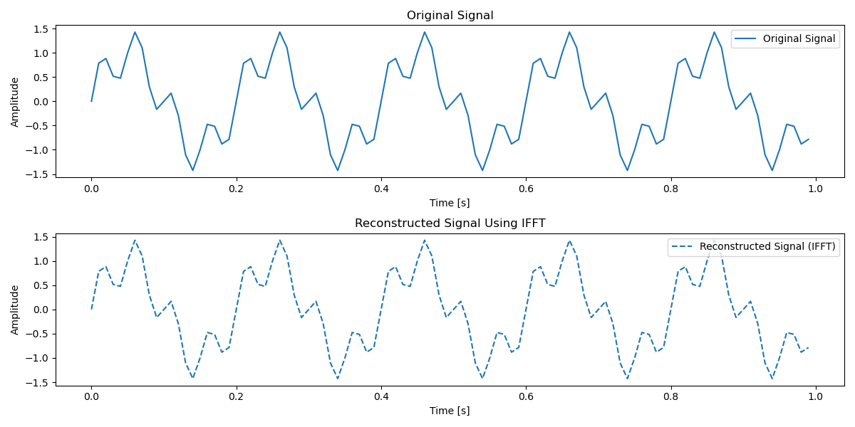
The Inverse Discrete Fast Fourier Transform (IDFT or IFFT) is the mathematical process that transforms a frequency-domain signal back into its time-domain representation. In SciPy this is implemented using the ifft function which efficiently computes the inverse of the Discrete Fourier Transform (DFT).

The IFFT is an essential tool for a wide range of signal processing applications by allowing for efficient and accurate reconstruction of signals from their frequency representations.

SciPy provides the scipy.fftpack.ifft or scipy.fft.ifft which is recommended function for calculating the inverse FFT.

Applications of IDFT

Here are the applications of the Inverse Discrete Fourier Transform −

• Signal Processing: It is used for converting frequency-domain data back to time-domain for analysis or visualization.
• Data Compression: It is used in conjunction with FFT to manipulate and compress signals.
• Filtering: Applying filters in the frequency domain and then transforming the filtered signal back to the time domain.

Example

Following is the example of using the Inverse Discrete Fast Fourier Transform with the help of Scipy −

import numpy as np
from scipy.fft import fft, ifft
import matplotlib.pyplot as plt

# Sample signal: A combination of two sine waves (5 Hz and 20 Hz)
sampling_rate = 100  # samples per second
T = 1.0 / sampling_rate  # sample spacing
t = np.linspace(0.0, 1.0, sampling_rate, endpoint=False)  # time vector
original_signal = np.sin(2.0 * np.pi * 5.0 * t) + 0.5 * np.sin(2.0 * np.pi * 20.0 * t)

# Compute the FFT of the signal
fft_result = fft(original_signal)

# Compute the IFFT to recover the original signal
reconstructed_signal = ifft(fft_result)

# Verify if the reconstructed signal matches the original
assert np.allclose(original_signal, reconstructed_signal.real), "Mismatch between original and reconstructed signal."

# Plot the original and reconstructed signals
plt.figure(figsize=(12, 6))

# Original Signal
plt.subplot(2, 1, 1)
plt.plot(t, original_signal, label='Original Signal')
plt.title("Original Signal")
plt.xlabel("Time [s]")
plt.ylabel("Amplitude")
plt.legend()

# Reconstructed Signal
plt.subplot(2, 1, 2)
plt.plot(t, reconstructed_signal.real, label='Reconstructed Signal (IFFT)', linestyle='--')
plt.title("Reconstructed Signal Using IFFT")
plt.xlabel("Time [s]")
plt.ylabel("Amplitude")
plt.legend()

plt.tight_layout()
plt.show()

Following is the output of the calculating the Discrete Fourier Transform(DFT) in Scipy −

Fast Fourier Transforms

SciPy's Fast Fourier Transform (FFT) routines are built to efficiently compute the Discrete Fourier Transform (DFT) and its inverse for one-, two-, and n-dimensional arrays. These routines find extensive use in signal processing, audio analysis, and image processing for analyzing data in the frequency domain.

Sr.No.	Function & Description
1	scipy.fft Computes the one-dimensional discrete Fourier Transform (DFT) using the Fast Fourier Transform (FFT) algorithm.
2	scipy.ifft Computes the inverse one-dimensional discrete Fourier Transform.
3	scipy.fft2 Computes the two-dimensional discrete Fourier Transform using FFT.
4	scipy.ifft2 Computes the inverse two-dimensional discrete Fourier Transform.
5	scipy.fftn Computes the n-dimensional discrete Fourier Transform.
6	scipy.ifftn Computes the inverse n-dimensional discrete Fourier Transform.
7	scipy.rfft Computes the one-dimensional real-input Fourier Transform.
8	scipy.irfft Computes the inverse one-dimensional real-input Fourier Transform.
9	scipy.rfft2 Computes the two-dimensional real-input Fourier Transform.
10	scipy.irfft2 Computes the inverse two-dimensional real-input Fourier Transform.
11	scipy.rfftn Computes the n-dimensional real-input Fourier Transform.
12	scipy.irfftn Computes the inverse n-dimensional real-input Fourier Transform.
13	scipy.hfft Computes the FFT of a real-valued signal using the Hermitian symmetry property.
14	scipy.ihfft Computes the inverse FFT of a real-valued signal assuming Hermitian symmetry.
15	scipy.hfft2 Computes the two-dimensional FFT for real-valued signals using Hermitian symmetry.
16	scipy.ihfft2 Computes the inverse two-dimensional FFT assuming Hermitian symmetry.
17	scipy.hfftn Computes the n-dimensional FFT for real-valued signals using Hermitian symmetry.
18	scipy.ihfftn Computes the inverse n-dimensional FFT assuming Hermitian symmetry.

Discrete Sin and Cosine Transforms

SciPy offers functions for the Discrete Cosine Transform (DCT) and Discrete Sine Transform (DST), which play a crucial role in areas like signal compression, image processing, and solving differential equations. These transformations are essential for representing and processing data efficiently.

Sr.No.	Function & Description
1	scipy.dct Computes the Discrete Cosine Transform (DCT), commonly used in signal and image processing.
2	scipy.idct Computes the inverse Discrete Cosine Transform.
3	scipy.dst Computes the Discrete Sine Transform (DST), useful in solving differential equations.
4	scipy.idst Computes the inverse Discrete Sine Transform.

Helper functions

The utility functions in SciPy help optimize Fourier Transform calculations by adjusting frequency components or managing parallel workers to improve processing speed. These tools significantly boost the efficiency and adaptability of Fourier analysis tasks.

Sr.No.	Function & Description
1	scipy.fhtoffset Computes the optimal offset for a Fast Hartley Transform (FHT).
2	scipy.next.fast.len Finds the next optimal input size for efficient FFT computation.
3	scipy.set.workers Sets the number of parallel workers for FFT computations.
4	scipy.get.workers Gets the current number of workers used for FFT computations.
5	scipy.fftshift Shifts the zero-frequency component of the Fourier Transform to the center.
6	scipy.ifftshift Reverses the effect of fftshift, moving the zero-frequency component back to the origin.
7	scipy.fftfreq Computes the sample frequencies for the discrete Fourier Transform.