SciPy - Discrete Probability Distributions

---

---

Discrete probability distributions refer to statistical models where the random variable can take a finite or countable set of values, often integers. These distributions are widely used in various fields like computer science, engineering and operations research to model phenomena such as successes in trials, event occurrences or sampling outcomes.

The scipy.stats library in Python provides an extensive collection of tools for working with these distributions, enabling us to calculate probability mass functions (PMF), cumulative distribution functions (CDF) and perform random sampling.

Key Discrete Distributions in SciPy

In SciPy, discrete distributions model random variables that can take specific values. SciPy provides a variety of discrete probability distributions along with methods for analyzing them.

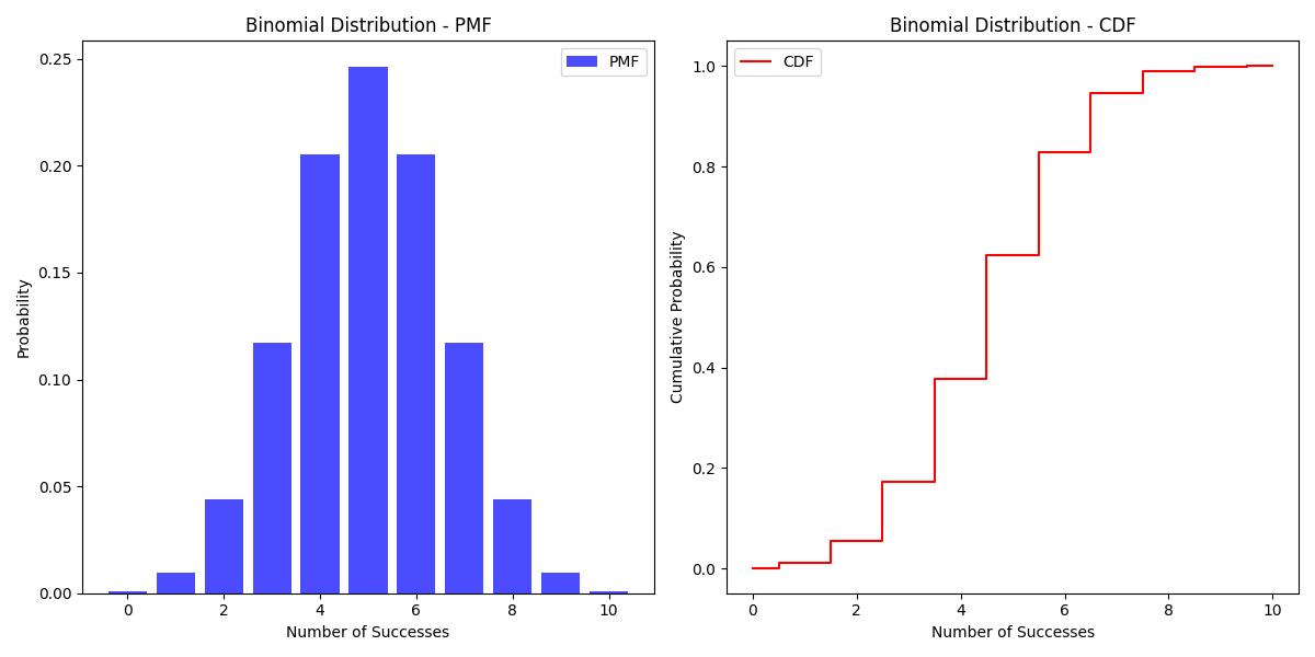
Binomial Distribution

The Binomial Distribution describes the number of successes in a specified number of independent trials where each trial has the same probability of success. It is frequently applied in scenarios such as coin toss experiments or quality control assessments.

In SciPy, the binomial distribution is represented by the scipy.stats.binom object. Below is an example which shows how to calculate and visualize the Probability Mass Function (PMF) and Cumulative Distribution Function (CDF) for a binomial distribution −

from scipy.stats import binom
import numpy as np
import matplotlib.pyplot as plt

# Parameters: n = trials, p = probability of success
n, p = 10, 0.5

# Generate an array of outcomes
x_values = np.arange(0, n + 1)

# Compute the PMF and CDF
pmf_values = binom.pmf(x_values, n, p)
cdf_values = binom.cdf(x_values, n, p)

# Plot the results
plt.figure(figsize=(12, 6))

# PMF plot
plt.subplot(1, 2, 1)
plt.bar(x_values, pmf_values, label='PMF', alpha=0.7, color='blue')
plt.title('Binomial Distribution - PMF')
plt.xlabel('Number of Successes')
plt.ylabel('Probability')
plt.legend()

# CDF plot
plt.subplot(1, 2, 2)
plt.step(x_values, cdf_values, label='CDF', color='red', where='mid')
plt.title('Binomial Distribution - CDF')
plt.xlabel('Number of Successes')
plt.ylabel('Cumulative Probability')
plt.legend()

plt.tight_layout()
plt.show()

Here is the output of the Binomial Distribution computed using the functions scipy.stats.binom.pmf() and scipy.stats.binom.cdf()−

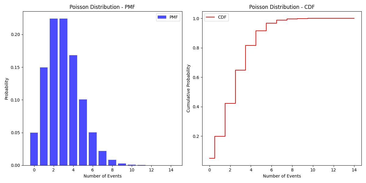
Poisson Distribution

The Poisson Distribution represents the count of events happening within a specific time or space interval by assuming the events occur independently and at a consistent average rate. It is commonly applied in areas like queueing systems, telecommunications and traffic analysis.

In SciPy the Poisson distribution is available through the scipy.stats.poisson() module. The following example shows how to compute and visualize the Probability Mass Function (PMF) and the Cumulative Distribution Function (CDF) for a Poisson distribution −

from scipy.stats import poisson
import numpy as np
import matplotlib.pyplot as plt

# Parameter: lambda (mean rate of events)
mu = 3

# Generate an array of outcomes
x_values = np.arange(0, 15)

# Compute the PMF and CDF
pmf_values = poisson.pmf(x_values, mu)
cdf_values = poisson.cdf(x_values, mu)

# Plot the results
plt.figure(figsize=(12, 6))

# PMF plot
plt.subplot(1, 2, 1)
plt.bar(x_values, pmf_values, label='PMF', alpha=0.7, color='blue')
plt.title('Poisson Distribution - PMF')
plt.xlabel('Number of Events')
plt.ylabel('Probability')
plt.legend()

# CDF plot
plt.subplot(1, 2, 2)
plt.step(x_values, cdf_values, label='CDF', color='red', where='mid')
plt.title('Poisson Distribution - CDF')
plt.xlabel('Number of Events')
plt.ylabel('Cumulative Probability')
plt.legend()

plt.tight_layout()
plt.show()

Below is the output of the Poisson distribution calculated using scipy.stats.poisson.pmf() and scipy.stats.poisson.cdf() function −

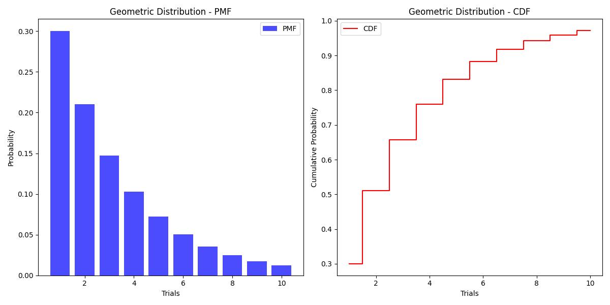
Geometric Distribution

The Geometric Distribution models the number of trials needed to get the first success in a series of independent Bernoulli trials in which each with a constant probability of success. This distribution is often used in areas like reliability testing and survival analysis.

In SciPy, the geometric distribution is represented by the scipy.stats.geom module. The following example illustrates how to compute and plot the Probability Mass Function (PMF) and Cumulative Distribution Function (CDF) for the geometric distribution −

from scipy.stats import geom
import numpy as np
import matplotlib.pyplot as plt

# Parameter: probability of success
p = 0.3

# Generate an array of outcomes
x_values = np.arange(1, 11)

# Compute the PMF and CDF
pmf_values = geom.pmf(x_values, p)
cdf_values = geom.cdf(x_values, p)

# Plot the results
plt.figure(figsize=(12, 6))

# PMF plot
plt.subplot(1, 2, 1)
plt.bar(x_values, pmf_values, label='PMF', alpha=0.7, color='blue')
plt.title('Geometric Distribution - PMF')
plt.xlabel('Trials')
plt.ylabel('Probability')
plt.legend()

# CDF plot
plt.subplot(1, 2, 2)
plt.step(x_values, cdf_values, label='CDF', color='red', where='mid')
plt.title('Geometric Distribution - CDF')
plt.xlabel('Trials')
plt.ylabel('Cumulative Probability')
plt.legend()

plt.tight_layout()
plt.show()

Here is the output of the geometric distribution calculated using scipy.stats.geom.pmf() and scipy.stats.geom.cdf() function −

Working with Discrete Distributions in SciPy

SciPy provides powerful methods to work with discrete distributions such as −

• PMF (Probability Mass Function): distribution.pmf(x, params) gives the probability of observing a specific outcome x.
• CDF (Cumulative Distribution Function): distribution.cdf(x, params) calculates the cumulative probability up to x.
• Random Sampling: distribution.rvs(params, size=N) generates N random values from the distribution.
• Mean and Variance: distribution.mean() and distribution.var() compute the mean and variance of the distribution.

For example the mean and variance of a Poisson distribution can be calculated as follows −

from scipy.stats import poisson

# Calculate the mean and variance of the Poisson distribution
mu = 3
mean = poisson.mean(mu)
variance = poisson.var(mu)

print("Mean of Poisson Distribution:", mean)
print("Variance of Poisson Distribution:", variance)

Below is the output of the mean and variance of the Poisson distribution −

Mean of Poisson Distribution: 3.0
Variance of Poisson Distribution: 3.0

With the scipy.stats module we can efficiently analyze and work with discrete probability distributions to solve a variety of real-world problems by ranging from modeling successes in trials to analyzing event occurrences.