SciPy - Distance Metrics

---

---

What are Distance Metrics?

In SciPy library distance metrics are crucial for measuring similarity or dissimilarity between two points in a given space. These metrics are widely used in fields such as machine learning, data analysis and clustering for tasks such as classification, clustering and nearest neighbor searches.

The scipy.spatial.distance module offers a variety of these metrics such as Euclidean, Manhattan, Cosine and Hamming distances, among others. Each metric serves different purposes for helping to determine the relationships and structures within datasets.

Types of Distance Metrics

As we know that the scipy.spatial.distance module provides a wide range of distance metrics with serving a different purpose as per the requirement. Below are the different Distance Metrics available in Scipy −

Euclidean Distance

In SciPy Euclidean distance is a measure of the straight-line distance between two points in Euclidean space. It is commonly used to quantify the similarity between two vectors by calculating the length of the shortest path connecting them.

The scipy.spatial.distance.euclidean() function is used to calculate the Euclidean Distance in Scipy.

Mathematically, it is defined as the square root of the sum of the squared differences between corresponding components of the two vectors. The formula is given as follows −

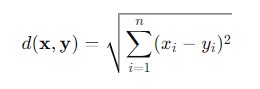
Where −

• x = (x₁, x₂, ....., x_n) and y = (y₁, y₂,....., y_n) − are the vectors representing the points in the space.
• (x_i, y_i) − is the difference between the x and y

Syntax

Following is the syntax of scipy.spatial.distance.euclidean() function −

scipy.spatial.distance.euclidean(u, v)

Parameters

Here are the Parameters of the scipy.spatial.distance.euclidean() function −

• u: The first point or vector in n-dimensional space.
• v: The second point or vector in n-dimensional space.

Return Value

This function returns the Euclidean distance between the points u and v.

Example

Following is a simple example showing how to compute the Euclidean distance between two points using SciPy's euclidean() function −

from scipy.spatial.distance import euclidean

# Define two points in 2D space
point1 = [1, 2]
point2 = [4, 6]

# Calculate the Euclidean distance between the two points
distance = euclidean(point1, point2)

print(f"Euclidean Distance: {distance}")

Following is the output of the Euclidean Distance calculated for two points −

Euclidean Distance: 5.0

Manhattan Distance

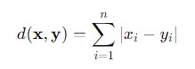
Manhattan Distance is also known as City-block Distance or L1 Norm which is a metric used to measure the distance between two points in a grid-like path. This is similar to how one would navigate a city grid.

Unlike Euclidean distance which measures the straight-line distance where as Manhattan distance calculates the total distance traveled along the grid lines.

Mathematically, the formula for calculating the Manhattan Distance −

Where −

• x = (x₁,x₂,.....,x_n) and y = (y₁,y₂,.....,y_n) − are the vectors representing the points.
• |x_i, y_i| − is the absolute difference between the x and y.

Syntax

Following is the syntax of scipy.spatial.distance.cityblock() function −

scipy.spatial.distance.cityblock(u, v)

Parameters

Here are the Parameters of the scipy.spatial.distance.cityblock() function −

• u: The first point or vector.
• v: The second point or vector.

Return Value

This function returns the City block distance between the vectors u and v.

Example

Here is the example which calculates the Manhattan Distance with the help of Scipy cityblock() function −

from scipy.spatial.distance import cityblock

# Define two vectors
vector1 = [1, 2, 3]
vector2 = [4, 6, 8]

# Calculate the City Block distance
distance = cityblock(vector1, vector2)

print(f"City Block Distance: {distance}")

Following is the output of the Cityblock Distance calculated for two points −

City Block Distance: 12

Minkowski Distance

Minkowski Distance is a generalization of both Euclidean and Manhattan distances and is used to measure the distance between two points in a normed vector space.

It provides a flexible framework by introducing a parameter p which determines the specific distance metric being used. Mathematically, the formula for calculating the Manhattan Distance −

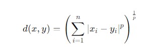
Where −

• x = (x₁, x₂ ,....., x_n) and y = (y₁, y₂,....., y_n) − are the vectors representing the points.
• |x_i, y_i| − is the absolute difference between the x and y.
• p − is a parameter that defines the distance metric.

Syntax

Following is the syntax of scipy.spatial.distance.minkowski() function −

scipy.spatial.distance.minkowski(u, v, p=2)

Parameters

Here are the Parameters of the scipy.spatial.distance.minkowski() function −

• u: The first point or vector which is an array of coordinates.
• v: The second point or vector which is an array of coordinates.
• p(float, optional): The power parameter for the Minkowski distance. Default is 2.

Note that,

When p = 1, it calculates the Manhattan Distance.

When p = 2, it calculates the Euclidean Distance.

When values of p > 2 measures a more general Minkowski distance.

Return Value

This function returns the Minkowski distance between the two points.

Example

Below is the example of finding the Minkowski distance between two points with the help of minkowski() function −

from scipy.spatial.distance import minkowski

# Define two points in 2D space
point1 = [1, 2]
point2 = [4, 6]

# Calculate Minkowski distance with p=3
distance = minkowski(point1, point2, p=3)

print(f"Minkowski Distance (p=3): {distance}")

Following is the output of the Minkowski Distance calculated for two points −

Minkowski Distance (p=3): 4.497941445275415

Chebyshev Distance

Chebyshev Distance is also known as the Maximum Metric or L Norm which is a distance metric used to measure the distance between two points in a grid-like system.

It is defined as the greatest of the absolute differences along any coordinate dimension. Mathematically the formula for calculating the Chebyshev Distance −

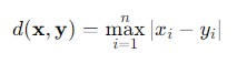
Where −

• x = (x₁,x₂,.....,x_n) and y = (y₁,y₂,.....,y_n) − are the vectors representing the points.
• |x_i,y_i| − is the absolute difference between the x and y.

Syntax

Following is the syntax of scipy.spatial.distance.chebyshev() function −

scipy.spatial.distance.chebyshev(u, v)

Parameters

Here are the Parameters of the scipy.spatial.distance.chebyshev() function −

• u: An array-like object representing the first point in the space.
• v: An array-like object representing the second point in the space.

Return Value

This function returns the Chebyshev distance between the two points u and v.

Example

Below is the example of finding the Chebyshev distance between two points with the help of Chebyshev() function −

from scipy.spatial.distance import chebyshev

# Define two points
point1 = [1, 2]
point2 = [4, 6]

# Calculate the Chebyshev distance
distance = chebyshev(point1, point2)

print(f"Chebyshev Distance: {distance}")

Following is the output of the Chebyshev Distance calculated for two points −

Chebyshev Distance: 4

Cosine Distance

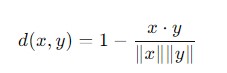
Cosine Distance is a measure of dissimilarity between two vectors based on the angle between them. It quantifies how different the vectors are by calculating the cosine of the angle between them with the distance being derived from this similarity measure.

It is often used in text analysis and clustering when the magnitude of the vectors is less important than their orientation. Mathematically the formula for calculating the Cosine Distance −

Syntax

Following is the syntax of scipy.spatial.distance.cosine() function −

scipy.spatial.distance.cosine(u, v)

Parameters

Here are the Parameters of the scipy.spatial.distance.cosine() function −

• u: An array-like object representing the first vector.
• v: An array-like object representing the second vector.

Return Value

This function returns the Cosine distance between the two points u and v.

Example

Below is the example of finding the Cosine distance between two points with the help of Cosine() function −

from scipy.spatial.distance import cosine

# Example vectors
vector1 = [1, 0, 1]
vector2 = [0, 1, 1]

# Compute Cosine distance
distance = cosine(vector1, vector2)

print(f"Cosine Distance: {distance}")

Following is the output of the Cosine Distance calculated for two points −

Cosine Distance: 0.5

Hamming Distance

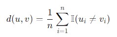
Hamming Distance is a measure of dissimilarity between two strings or binary vectors of equal length. It quantifies the number of positions at which the corresponding elements differ.

It is often used in error detection and correction algorithms as well as in various applications involving binary data.

A Hamming distance of 0 indicates that the vectors are identical while a distance closer to 1 indicates more dissimilarity. Mathematically the formula for calculating the Hamming Distance −

Syntax

Following is the syntax of scipy.spatial.distance.hamming() function −

scipy.spatial.distance.hamming(u, v)

Parameters

Here are the Parameters of the scipy.spatial.distance.hamming() function −

• u: An array-like object or list representing the first vector or string.
• v: An array-like object or list representing the second vector or string.

Return Value

This function returns the Hamming distance between the two points u and v.

Example

In this example the Hamming distance represents the fraction of positions where the two binary vectors differ −

from scipy.spatial.distance import hamming

# Example binary vectors
vector1 = [1, 0, 1, 0, 1]
vector2 = [1, 1, 0, 0, 1]

# Compute Hamming distance
distance = hamming(vector1, vector2)

print(f"Hamming Distance: {distance}")

Below is the output of the Hamming Distance calculated for two points −

Hamming Distance: 0.4

Jaccard Distance

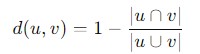
Jaccard Distance is a measure of dissimilarity between two sets. It is calculated as one minus the Jaccard similarity coefficient which is the ratio of the size of the intersection of the sets to the size of their union.

Jaccard distance is often used in binary or categorical data analysis which is particularly in fields like clustering and classification.

In SciPy library the Jaccard distance can be computed using the scipy.spatial.distance.jaccard() function. Mathematically the formula for calculating the Jaccard Distance −

Where −

• |u∩v|: is the size of the intersection of the two sets.
• |u∪ ∪ v|: is the size of the union of the two sets.

Syntax

Following is the syntax of scipy.spatial.distance.jaccard() function −

scipy.spatial.distance.jaccard(u, v)

Parameters

Here are the Parameters of the scipy.spatial.distance.jaccard() function −

• u: An array-like object representing the first binary vector or set.
• v: An array-like object representing the second binary vector or set.

Return Value

This function returns the Jaccard distance between the two points u and v.

Example

Following is the example of using the jaccard() function to calculate the Jaccard Distance in SciPy −

from scipy.spatial.distance import jaccard

# Example binary vectors
vector1 = [1, 0, 1, 0, 1, 1]
vector2 = [0, 1, 1, 0, 1, 0]

# Compute Jaccard distance
distance = jaccard(vector1, vector2)

print(f"Jaccard Distance: {distance}")

Following is the output of the Jaccard Distance calculated for two points −

Jaccard Distance: 0.6

Canberra Distance

Canberra Distance is a metric that measures the dissimilarity between two points by summing the absolute differences between their coordinates and normalized by the sum of their absolute values.

• It is particularly sensitive to differences when both coordinates are small by making it useful for cases where values can be zero or near-zero.
• The Canberra distance is often used in various fields such as environmental science and economics where proportional differences are more significant than absolute differences.

Mathematically the formula for calculating the Canberra Distance is given as follows −

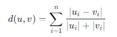
• |u_i-v_i| − is the absolute difference between the u and v.
• |u_i|+|v_i| − is the sum of the absolute values of the th coordinates.

Syntax

Following is the syntax of scipy.spatial.distance.canberra() function −

scipy.spatial.distance.canberra(u, v)

Parameters

Here are the Parameters of the scipy.spatial.distance.canberra() function −

• u: An array-like object representing the first vector.
• v: An array-like object representing the second vector.

Return Value

This function returns the Canberra distance between the two points u and v.

Example

Following is the example of using the canberra() function to calculate the Canberra Distance in SciPy −

from scipy.spatial.distance import canberra

# Example vectors
vector1 = [10, 20, 30]
vector2 = [15, 24, 36]

# Compute Canberra distance
distance = canberra(vector1, vector2)

print(f"Canberra Distance: {distance}")

Below is the output of the Canberra Distance calculated for two points −

Canberra Distance: 0.38181818181818183

Bray-Curtis Distance

Bray-Curtis Distance is a measure of dissimilarity between two non-negative numerical vectors which often used in ecology and biology for comparing species abundances.

It quantifies the difference between two samples by taking into account the magnitude of their elements by making it particularly useful for datasets where the absolute differences are more important than their relative differences.

In SciPy the Bray-Curtis distance can be calculated using the scipy.spatial.distance.braycurtis() function.

Mathematically the formula for calculating the Canberra Distance is given as follows −

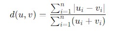
Where −

• |u_i-v_i| − is the absolute difference between the corresponding elements of vectors u and v.
• u_i+v_i − is the sum of the corresponding elements.

Syntax

Following is the syntax of scipy.spatial.distance.braycurtis() function −

scipy.spatial.distance.braycurtis(u, v)

Parameters

Here are the Parameters of the scipy.spatial.distance.braycurtis() function −

• u: An array-like object representing the first vector.
• v: An array-like object representing the second vector.

Return Value

This function returns the Bray-Curtis distance between the two points u and v.

Example

Here is the example of using the braycurtis() function to calculate the Bray-Curtis Distance in SciPy −

from scipy.spatial.distance import braycurtis

# Example vectors
vector1 = [1, 3, 5, 7]
vector2 = [2, 4, 6, 8]

# Compute Bray-Curtis distance
distance = braycurtis(vector1, vector2)

print(f"Bray-Curtis Distance: {distance}")

Below is the output of the Canberra Distance calculated for two points −

Bray-Distance: 0.1111111111111111