Scipy Double Integration (dblquad)

---

---

Double integration in SciPy

In SciPy Double Integration is performed using the dblquad() function which allows us to compute the integral of a function of two variables over a specified region. This function integrates over two dimensions by evaluating the inner integral first with respect to one variable and then the outer integral with respect to the second variable.

The limits of integration can be constants or functions by providing flexibility in defining the integration region. Double integration is useful for calculating areas, volumes and solving partial differential equations.

In Mathematics, Double Integration is a process of integrating a function of two variables over a specified region in the xy-plane. The double integral of a function f(x,y) over the rectangular region defined by a x b and g(x) y h is given as follows −

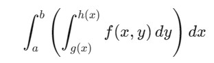
The inner integral is evaluated first with respect to y while holding x constant. The result is then integrated with respect to x,over the limits a and b.

Syntax

Following is the syntax of dblquad() function in scipy.integrate module to calculate the Double Integration −

scipy.integrate.dblquad(func, a, b, gfun, hfun, args=(), epsabs=1.49e-08, epsrel=1.49e-08)

Parameters

Below are the parameters of the dblquad() function in scipy.integrate module −

• func: The function to be integrated. It will take two arguments (x, y).
• a: The lower limit of integration for the outer integral with respect to x.
• b: The upper limit of integration for the outer integral with respect to x.
• gfun: A function that returns the lower limit of integration for the inner integral with respect to y.
• hfun: A function that returns the upper limit of integration for the inner integral with respect to y.
• args(optional): Extra arguments to pass to func.
• epsabs: Absolute tolerance with the default value 1.4910^-8
• epsrel: Relative tolerance with the default value 1.4910^-8

Example of Double Integration

Following is the example of calculating the Double Integartion of the given function f(x,y) = x.y over the regions, x ranges from 0 to 1 and y ranges from 0 to 2x.

import scipy.integrate as integrate

# Define the function to integrate: f(x, y) = x * y
def integrand(y, x):
    return x * y

# Perform double integration using scipy.integrate.dblquad
result, error = integrate.dblquad(integrand, 0, 1, lambda x: 0, lambda x: 2*x)

# Print the result and error
print("Result of the double integration:", result)
print("Estimated error:", error)

Following is the output of the Double Integration of the given function using dblquad() −

Result of the double integration: 0.5
Estimated error: 2.2060128823111155e-14

Handling Limits

In scipy.integrate.dblquad() we can handle infinite limits by passing scipy.inf or -scipy.inf for the integration bounds. This allows us to perform integrals over unbounded regions. The dblquad() function internally handles these infinite limits using numerical techniques suited for improper integrals.

Example

Below is the example of handling the limits of the functions f(x,y) = e^-x2-y2 over infinite region where x ranges from 0 to infinity () and y ranges from 0 to infinity () −

import numpy as np
import scipy.integrate as integrate

# Define the function to integrate: f(x, y) = exp(-x^2 - y^2)
def integrand(y, x):
    return np.exp(-x**2 - y**2)

# Perform double integration with infinite limits
result, error = integrate.dblquad(integrand, 0, np.inf, lambda x: 0, lambda x: np.inf)

# Print the result and error
print("Result of the double integration:", result)
print("Estimated error:", error)

Following is the output of handling limits when using the dblquad() function −

Result of the double integration: 0.7853981633973343
Estimated error: 1.4647640380321503e-08

Error Tolerance

In the scipy.integrate.dblquad() function the error tolerance is controlled through two parameters namely, epsabs and epsrel. These parameters help us to define the accuracy of the result by setting the absolute and relative error tolerances.

The integration routine tries to balance both absolute and relative error tolerance criteria. It ensures that the result is accurate either by meeting the absolute error or relative error conditions.

Example

Here is the example of handling the error tolerance in calculating the double integration with the help of dblquad() function −

import numpy as np
import scipy.integrate as integrate

# Define the function to integrate: f(x, y) = exp(-x^2 - y^2)
def integrand(y, x):
    return np.exp(-x**2 - y**2)

# Perform double integration with custom error tolerances
result, error = integrate.dblquad(integrand, 0, np.inf, lambda x: 0, lambda x: np.inf, epsabs=1e-10, epsrel=1e-10)

# Print the result and error
print("Result of the double integration:", result)
print("Estimated error:", error)

Following is the output of error tolerance used in dblquad() function −

Result of the double integration: 0.785398163397448
Estimated error: 9.688368546159476e-

Complex Functions

Here is the example of calculating the double integration of the complex function f(x,y) = e^-(x2+y2)+i.sin(x+y) −

import numpy as np
import scipy.integrate as integrate

# Define the real part of the function: exp(-x^2 - y^2)
def real_part(y, x):
    return np.exp(-x**2 - y**2)

# Define the imaginary part of the function: sin(x + y)
def imag_part(y, x):
    return np.sin(x + y)

# Define finite bounds to replace infinity, for instance (0, 100)
finite_bound = 100

# Perform double integration for real part
real_result, real_error = integrate.dblquad(real_part, 0, finite_bound, lambda x: 0, lambda x: finite_bound)

# Perform double integration for imaginary part
imag_result, imag_error = integrate.dblquad(imag_part, 0, finite_bound, lambda x: 0, lambda x: finite_bound)

# Combine the real and imaginary parts into a complex number
complex_result = real_result + 1j * imag_result

# Print the result
print("Result of the double integration (complex):", complex_result)
print("Estimated error (real part):", real_error)
print("Estimated error (imaginary part):", imag_error)

Following is the output of calculating the double integration of a complex function using dblquad() function −

Result of the double integration (complex): (0.7853981633971309-0.13943398500584472j)
Estimated error (real part): 1.1078396381028211e-08
Estimated error (imaginary part): 1.4892850109719667e-08