Scipy Fast Fourier Transform (FFT)

The Fast Fourier Transform (FFT) in SciPy is a powerful algorithm designed to compute the Discrete Fourier Transform (DFT) and its inverse with high efficiency, significantly reducing the computational cost compared to the standard DFT.

This allows for the conversion of signals between the time and frequency domains by enabling various types of signal and data analysis.

Scipy Fast Fourier Transform in SciPy

SciPy's scipy.fft module offers a suite of functions for performing one-dimensional, two-dimensional and even multi-dimensional FFTs. The primary function scipy.fft.fft is used for computing the one-dimensional FFT of an input array while scipy.fft.ifft calculates the inverse FFT by converting frequency data back to the time domain.

For data sets that consist of real numbers we can use scipy.fft.rfft and scipy.fft.irfft are optimized versions that only handle positive frequencies by reducing both computational time and memory usage.

For more complex data the functions such as scipy.fft.fftn and scipy.fft.ifftn extend these capabilities to multi-dimensional arrays which is particularly useful for tasks such as image processing.

SciPys FFT functions also provide flexibility with features such as normalization, axis specification and zero-padding. Moreover scipy.fft.fftshift and scipy.fft.ifftshift are useful for shifting the zero-frequency component to the center or moving it back to the edges by aiding in frequency spectrum visualization.

Key Features of Fast Fourier Transform(FFT)

The features make FFT a versatile and powerful tool for various applications such as signal processing, image analysis and audio processing. Following are the key features of Fast Fourier Transform(FFT) −

• Efficiency: FFT dramatically reduces the computational complexity of calculating the Discrete Fourier Transform (DFT) from O(N)² to O(N log N) by making it much faster for large datasets.
• Signal Analysis: The FFT transforms time-domain signals into their frequency-domain representation by enabling the analysis of different frequency components in the signal.
• Inverse FFT (IFFT): The inverse FFT function reconstructs the original time-domain signal from its frequency-domain components.
• Support for Real and Complex Inputs: FFT can handle both real-valued and complex-valued data. Specialized versions such as rfft for real-valued inputs further optimize performance.
• Multi-Dimensional FFTs: The Functions such as fftn and ifftn allow FFT to be applied to multi-dimensional data such as images or volumetric data by making it useful in image and 3D data analysis.
• Zero-Padding and Truncation: Zero-padding is used to increase the resolution of the frequency spectrum while truncation can be used to reduce computational costs for signals with significant zeros.
• Frequency Shifting: Functions such as fftshift and ifftshift shift the zero-frequency component to the center or back by facilitating better visualization of the frequency spectrum.
• Normalization Options: Various normalization options ensure accurate scaling of the FFT results according to different conventions.

Example 1

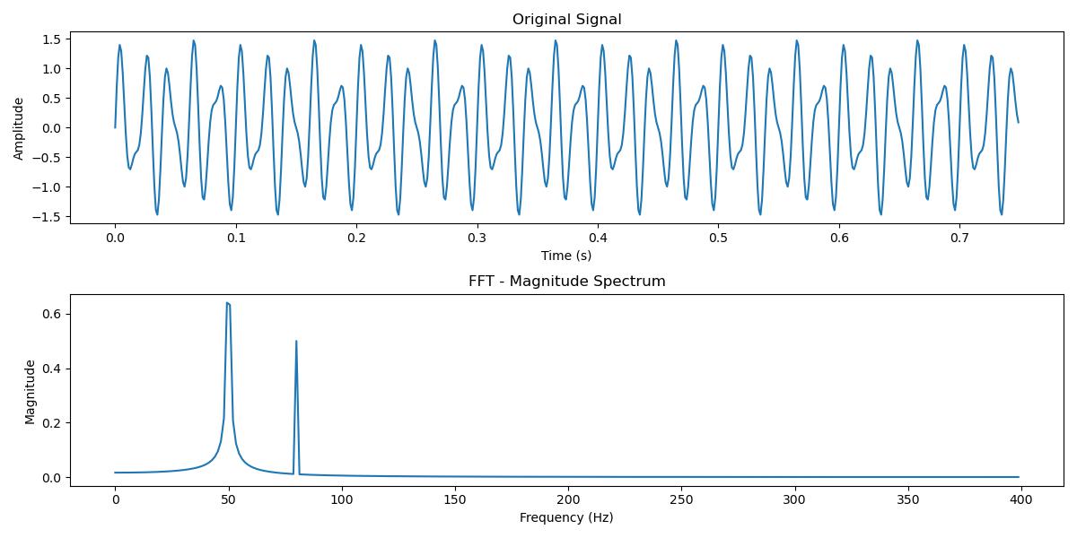
Heres a simple example of using SciPy to compute the one-dimensional Fast Fourier Transform (FFT) of a signal along with its visualization −

import numpy as np
from scipy.fft import fft, ifft
import matplotlib.pyplot as plt

# Create a sample signal
N = 600  # Number of sample points
T = 1.0 / 800.0  # Sample spacing
x = np.linspace(0.0, N*T, N, endpoint=False)
# Create a signal composed of two different frequencies
y = np.sin(50.0 * 2.0*np.pi*x) + 0.5*np.sin(80.0 * 2.0*np.pi*x)

# Compute the FFT
yf = fft(y)

# Compute the corresponding frequencies
xf = np.fft.fftfreq(N, T)[:N//2]

# Plot the original signal
plt.figure(figsize=(12, 6))

plt.subplot(2, 1, 1)
plt.plot(x, y)
plt.title("Original Signal")
plt.xlabel("Time (s)")
plt.ylabel("Amplitude")

# Plot the FFT (magnitude spectrum)
plt.subplot(2, 1, 2)
plt.plot(xf, 2.0/N * np.abs(yf[:N//2]))
plt.title("FFT - Magnitude Spectrum")
plt.xlabel("Frequency (Hz)")
plt.ylabel("Magnitude")

plt.tight_layout()
plt.show()

Following is the output of the 1-Dimensional Fast Fourier Transform(FFT) −

Example 2

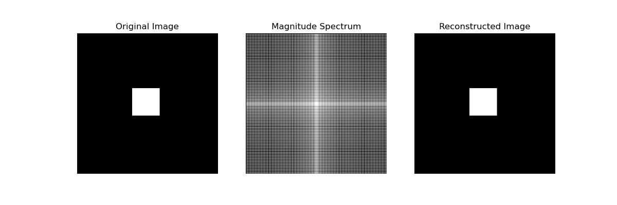
Heres a simple example of performing a two-dimensional Fast Fourier Transform (2D FFT) using SciPy. This example shows how to transform a 2D image or any 2D array into the frequency domain and then back into the spatial domain using the inverse 2D FFT −

import numpy as np
import matplotlib.pyplot as plt
from scipy.fft import fft2, ifft2, fftshift

# Create a sample 2D array (image)
image = np.zeros((256, 256))
image[100:150, 100:150] = 255  # Create a white square in the middle

# Compute the 2D FFT
fft_image = fft2(image)

# Shift the zero frequency component to the center of the spectrum
fft_image_shifted = fftshift(fft_image)

# Compute the magnitude spectrum
magnitude_spectrum = np.abs(fft_image_shifted)

# Inverse 2D FFT to reconstruct the original image
reconstructed_image = ifft2(fft_image).real

# Plot the original image, magnitude spectrum, and reconstructed image
plt.figure(figsize=(12, 4))

# Original image
plt.subplot(1, 3, 1)
plt.title("Original Image")
plt.imshow(image, cmap='gray')
plt.axis('off')

# Magnitude spectrum
plt.subplot(1, 3, 2)
plt.title("Magnitude Spectrum")
plt.imshow(np.log(magnitude_spectrum + 1), cmap='gray')
plt.axis('off')

# Reconstructed image
plt.subplot(1, 3, 3)
plt.title("Reconstructed Image")
plt.imshow(reconstructed_image, cmap='gray')
plt.axis('off')

plt.show()

Here is the output of the 2d-Dimensional Fast Fourier Transform(FFT) −

Applications of FFT

The Fast Fourier Transform (FFT) in SciPy has a wide range of applications across various fields due to its ability to efficiently convert time-domain signals into their frequency-domain representation. Here are some key applications of FFT −

• Signal Processing: FFT is used to analyze the frequency content of signals, detect patterns, filter noise and design digital filters. It's fundamental in telecommunications, audio signal processing and radar signal analysis.
• Image Processing: FFT helps in image filtering, enhancement and compression by transforming images to the frequency domain by enabling operations such as high-pass and low-pass filtering.
• Audio Analysis: FFT is used for pitch detection, sound synthesis and music analysis. It helps in extracting features such as spectral content and rhythm from audio signals.
• Vibration Analysis: In mechanical engineering the FFT is used to analyze vibration data from machines to identify faults and predict maintenance needs.
• Medical Imaging: FFT is used in MRI and other imaging techniques to reconstruct images from raw data, improve resolution and filter noise.
• Astronomy: FFT is employed to analyze the frequency spectrum of astronomical signals by helping in the detection and characterization of celestial objects.