SciPy - Generating Random Samples

---

---

Generating random samples in SciPy refers to the process of drawing values from predefined probability distributions using the scipy.stats module. SciPy provides a wide range of continuous and discrete probability distributions such as the normal, uniform, binomial and exponential distributions. The .rvs() (random variates) method is used to generate these samples while maintaining the statistical properties of the chosen distribution.

Mathematically, a random sample X is drawn from a probability distribution f(x) where,

X  f(x,)

Here represents the parameters of the distribution such as mean and standard deviation for a normal distribution.

Random sampling is essential in simulations, statistical modeling and machine learning. It allows researchers to approximate real-world uncertainties, perform Monte Carlo simulations and conduct hypothesis testing.

Here are the key parameters in include −

• loc: Represents the mean or starting value of the distribution.
• scale: Controls the spread or range.
• size: Specifies the number of samples to generate.
• random_state: Ensures reproducibility by fixing the random seed.

For example norm.rvs(loc=0, scale=1, size=10) generates 10 random numbers from a standard normal distribution. This functionality makes SciPy a powerful tool for probabilistic data analysis and simulations.

Generating Random Samples from Different Distributions

SciPy provides powerful tools for generating random samples from various probability distributions through the scipy.stats module. This is widely used in statistical analysis, simulations and machine learning.

Normal (Gaussian) Distribution

The Normal distribution is also known as the Gaussian distribution which is one of the most important probability distributions in statistics. It is widely used in real-world applications such as finance, physics, biology and machine learning.

SciPy provides the norm.rvs() function within scipy.stats module to generate random samples from a normal distribution.

Syntax

Following is the syntax of SciPy's norm.rvs() function which is used to generate random samples from a normal distribution −

scipy.stats.norm.rvs(loc=mean, scale=std_dev, size=n, random_state=seed)

parameters

Here are the parameters of the function scipy.stats.norm.rvs() −

• loc: The Mean () of the distribution.
• scale: The Standard deviation () of the distribution.
• size: The number of random samples to generate.
• random_state: An optional seed for reproducibility.

Example

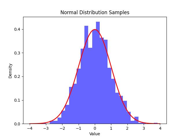
Following is the example in which we generate 1,000 random samples from a normal distribution with a mean of 0 and a standard deviation of 1. The histogram of the samples is plotted alongside the theoretical probability density function (PDF) to illustrate the distribution −

import numpy as np
import matplotlib.pyplot as plt
from scipy.stats import norm

# Parameters
 = 0    # Mean
 = 1    # Standard deviation
n = 1000 # Number of samples

# Generate random samples
samples = norm.rvs(loc=, scale=, size=n, random_state=42)

# Plot histogram
plt.hist(samples, bins=30, density=True, alpha=0.6, color='b')

# Plot the theoretical PDF
x = np.linspace(-4, 4, 100)
plt.plot(x, norm.pdf(x, loc=, scale=), 'r', lw=2)

plt.title("Normal Distribution Samples")
plt.xlabel("Value")
plt.ylabel("Density")
plt.show()

Following is the output of the random samples generated from Normal Distribution −

Uniform Distribution

The Uniform distribution is a probability distribution where all outcomes are equally likely within a given range. It is commonly used in simulations, random sampling and statistical modeling.

SciPy provides the uniform.rvs() function within the scipy.stats module to generate random samples from a uniform distribution.

Syntax

Following is the syntax of SciPy's uniform.rvs() function which is used to generate random samples from a uniform distribution −

scipy.stats.uniform.rvs(loc=a, scale=b-a, size=n, random_state=seed)

parameters

Here are the parameters of the function scipy.stats.uniform.rvs() −

• loc: The lower bound (a) of the distribution.
• scale: The range (b - a) of the distribution.
• size: The number of random samples to generate.
• random_state: An optional seed for reproducibility.

Example

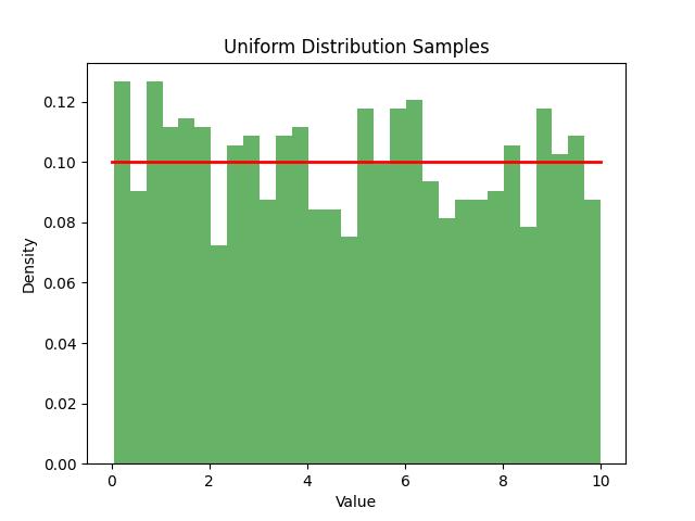
Following is the example in which we generate 1,000 random samples from a uniform distribution between 0 and 10. The histogram of the samples is plotted alongside the theoretical probability density function (PDF) to illustrate the distribution −

import numpy as np
import matplotlib.pyplot as plt
from scipy.stats import uniform

# Parameters
a = 0    # Lower bound
b = 10   # Upper bound
n = 1000 # Number of samples

# Generate random samples
samples = uniform.rvs(loc=a, scale=b-a, size=n, random_state=42)

# Plot histogram
plt.hist(samples, bins=30, density=True, alpha=0.6, color='g')

# Plot the theoretical PDF
x = np.linspace(a, b, 100)
plt.plot(x, uniform.pdf(x, loc=a, scale=b-a), 'r', lw=2)

plt.title("Uniform Distribution Samples")
plt.xlabel("Value")
plt.ylabel("Density")
plt.show()

Below is the output of the random samples generated from Uniform Distribution −

Exponential Distribution

The Exponential distribution is a continuous probability distribution that describes the time between events in a Poisson process where events occur independently at a constant average rate. It is widely applied in reliability engineering, queuing systems and survival analysis.

SciPy provides the expon.rvs() function within the scipy.stats module to generate random samples following an exponential distribution.

Syntax

The following is the syntax for SciPy's expon.rvs() function, which is used to generate random samples from an exponential distribution −

scipy.stats.expon.rvs(scale=1/lambda, size=n, random_state=seed)

Parameters

The scipy.stats.expon.rvs() function accepts the following parameters −

• scale: The reciprocal of the rate parameter (1/), which defines the mean time between events.
• size: The number of random samples to be generated.
• random_state: Optional seed value to ensure reproducibility of results.

Example

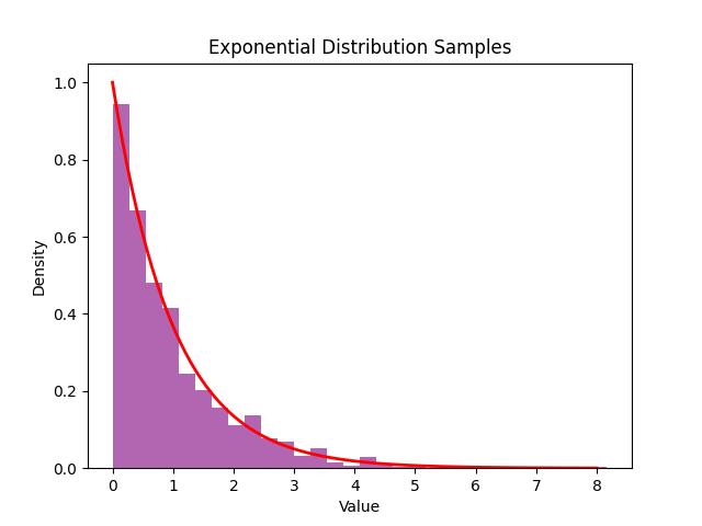
Below is the example which helps, how to generate 1,000 random samples from an exponential distribution with a rate parameter () of 1. The histogram of the samples is plotted along with the probability density function (PDF) to visualize the distribution −

import numpy as np
import matplotlib.pyplot as plt
from scipy.stats import expon

# Define parameters
 = 1    # Rate parameter
n = 1000 # Number of samples

# Generate random samples
samples = expon.rvs(scale=1/, size=n, random_state=42)

# Plot histogram
plt.hist(samples, bins=30, density=True, alpha=0.6, color='purple')

# Plot the theoretical PDF
x = np.linspace(0, 8, 100)
plt.plot(x, expon.pdf(x, scale=1/), 'r', lw=2)

plt.title("Exponential Distribution Samples")
plt.xlabel("Value")
plt.ylabel("Density")
plt.show()

Here is the output which gives the random samples generated from the Exponential Distribution −

Binomial Distribution

The Binomial distribution is a probability distribution that represents the number of successful outcomes in a fixed number of independent trials. Each trial results in one of two possible outcomes: success or failure, with a constant probability of success.

This distribution is commonly applied in real-world scenarios where outcomes are binary such as evaluating product defects in a manufacturing process or counting how many times a coin lands on heads in multiple tosses.

In SciPy, the binom.rvs() function, available within the scipy.stats module, allows users to generate random values that follow a binomial pattern.

Syntax

The following is the syntax for the binom.rvs() function, which is used to create random values that follow a binomial pattern −

scipy.stats.binom.rvs(n=trials, p=probability, size=samples, random_state=seed)

Parameters

The function binom.rvs() includes several input parameters as mentioned follows −

• n: Represents the number of trials or attempts.
• p: The probability of achieving success in a single trial.
• size: Specifies the number of random values to generate.
• random_state: An optional parameter to set a fixed seed for reproducibility.

Example

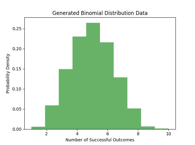
In the following example we create 1,000 random values from a binomial distribution where there are 10 trials, and the probability of success in each trial is 0.5. The generated values are then displayed using a histogram to show the distribution pattern −

import numpy as np
import matplotlib.pyplot as plt
from scipy.stats import binom

# Define the parameters
num_trials = 10   # Number of experiments
success_prob = 0.5  # Probability of success per trial
num_samples = 1000  # Total samples to generate

# Generate the binomially distributed random values
data = binom.rvs(n=num_trials, p=success_prob, size=num_samples, random_state=42)

# Plot a histogram of the generated values
plt.hist(data, bins=10, density=True, alpha=0.6, color='g')

plt.title("Generated Binomial Distribution Data")
plt.xlabel("Number of Successful Outcomes")
plt.ylabel("Probability Density")
plt.show()

Following is the output which represents the binomially distributed random samples −

Poisson distribution

The Poisson distribution is a statistical model that represents the frequency of an event occurring within a fixed period of time or space. It is applicable in scenarios where occurrences are random, independent and happen at a constant average rate.

This distribution is commonly used in real-world cases such as estimating the number of customer calls received by a support center per hour by tracking the footfall at a store within a set duration or analyzing the frequency of emails arriving in an inbox daily.

In SciPy, the poisson.rvs() function from the scipy.stats module allows users to generate random samples that follow a Poisson distribution.

Syntax

The following is the syntax for the poisson.rvs() function which generates random values following a Poisson distribution −

scipy.stats.poisson.rvs(mu=rate, size=samples, random_state=seed)

Parameters

The function poisson.rvs() includes several input parameters as mentioned follows −

• mu: The expected number of occurrences (mean rate of events).
• size: Specifies the number of random values to generate.
• random_state: An optional parameter to set a fixed seed for reproducibility.

Example

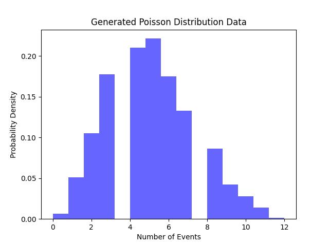
Here in this example we generate 1,000 random values from a Poisson distribution with an average event rate of 5 per unit time. The generated values are then displayed using a histogram to illustrate the distribution pattern −

import numpy as np
import matplotlib.pyplot as plt
from scipy.stats import poisson

# Define the parameters
event_rate = 5   # Average occurrences per time unit
num_samples = 1000  # Total samples to generate

# Generate Poisson-distributed random values
data = poisson.rvs(mu=event_rate, size=num_samples, random_state=42)

# Plot a histogram of the generated values
plt.hist(data, bins=15, density=True, alpha=0.6, color='b')

plt.title("Generated Poisson Distribution Data")
plt.xlabel("Number of Events")
plt.ylabel("Probability Density")
plt.show()

The following graph represents the Poisson-distributed random samples −

Setting a Seed for Reproducibility

When generating random numbers in Python then the output changes with each execution. This can be problematic for debugging, testing or sharing results. To ensure consistency we use a seed value to initialize the random number generator. This makes the random output reproducible across multiple runs.

In SciPy, functions like binom.rvs() for generating binomially distributed random values include the random_state parameter. Setting this parameter to a fixed integer ensures that the generated values remain the same each time the code is executed.

Example

The following example demonstrates how setting a seed ensures that the same random values are generated in multiple runs:

import numpy as np
import matplotlib.pyplot as plt
from scipy.stats import binom

# Define parameters
num_trials = 10    # Number of experiments
success_prob = 0.5  # Probability of success per trial
num_samples = 10   # Total samples to generate

# Generate random values with a fixed seed
seed_value = 42
samples1 = binom.rvs(n=num_trials, p=success_prob, size=num_samples, random_state=seed_value)
samples2 = binom.rvs(n=num_trials, p=success_prob, size=num_samples, random_state=seed_value)

# Display the results
print("First Run:", samples1)
print("Second Run:", samples2)

# Verify if both runs produce the same output
print("Are both runs identical?", np.array_equal(samples1, samples2))

The output will confirm that setting a seed generates the same values every time −

First Run: [4 8 6 5 3 3 3 7 5 6]
Second Run: [4 8 6 5 3 3 3 7 5 6]
Are both runs identical? True