SciPy - Grid Data Multi-Dimensional Interpolation

---

---

Grid Data Multi-Dimensional Interpolation

SciPy Grid Data Multi-Dimensional Interpolation is a technique used to estimate the values of a function at arbitrary points in multi-dimensional space based on data that is known only at a finite set of points. This method is particularly useful when dealing with irregularly spaced data in applications such as geographic data analysis, image processing and scientific simulations.

In SciPy the core function for this type of interpolation is scipy.interpolate.griddata() function. It supports multiple interpolation methods including nearest-neighbor, linear and cubic interpolation by allowing users to balance between accuracy and computational efficiency. The griddata() function works for datasets of any dimensionality by making it a flexible tool for multi-dimensional data interpolation.

Syntax

Following is the syntax of griddata() function which is used to perform Grid Data Mutli- Dimensional Interpolation in scipy −

scipy.interpolate.griddata(
   points, 
   values, 
   xi, 
   method='linear', 
   fill_value=np.nan, 
   rescale=False
)

Parameters

Here are the parameters of the function griddata() −

• points: An array of shape (n, D) where n is the number of known data points and D is the number of dimensions. Each row represents the coordinates of a known data point.
• values: An array of length n containing the values corresponding to each point in points.
• xi: The coordinates at which to interpolate the data. This can be a single point or an array of points. Its shape can be (m, D) where m is the number of points at which interpolation is desired.
• method: The interpolation method to use such as linear, nearest, cubic. The default value is linear.
• fill_value: Value to return for points outside the convex hull of the input points. This is useful for managing out-of-bounds queries.
• rescale: If this parameter set to True then the input points will be re-scaled to fit in the unit box before interpolation. This is particularly useful when the ranges of the dimensions of the input points differ significantly.

Key Grid Data Interpolation Methods in Scipy

In SciPy the griddata() function offers three primary interpolation methods for grid data. These methods are useful for interpolating scattered data points over a grid in one or more dimensions. Let's see them one by one in detail −

Linear Interpolation in griddata()

Linear interpolation in griddata() is a method that estimates unknown values within the bounds of known data points using linear equations. It is widely used when scattered data points are provided and an interpolated surface or function is desired.

n the view of multi-dimensional interpolation with SciPys griddata() the linear interpolation is used to compute values at new points based on the values of surrounding points by forming a surface composed of triangular facets.

Following are the key features of Linear interpolation in griddata() −

• Method: For 2D interpolation, the linear interpolation involves creating triangles in 2D between neighboring points and for higher dimensions. It constructs simplified generalized triangles.
• Interpolation: The value at any new point is calculated based on a weighted average of the values at the vertices of the surrounding simplex. This provides a simple linear interpolation of the data.
• Boundary Conditions: Linear interpolation assumes the function is well-behaved within the bounds of the known data points and does not extrapolate outside the convex hull of the input points.

To use the linear method in Grid Data Multi Dimensional Interpolation we have to pass the argument method = 'linear' for griddata() function. Here is the syntax −

griddata(points, values, xi, method='linear')

Example

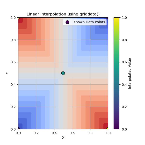
Heres a simple example of linear interpolation using SciPy's griddata() function where we interpolate values at new points based on known data points in 2D space −

import numpy as np
import matplotlib.pyplot as plt
from scipy.interpolate import griddata

# Define known data points (in 2D) and their corresponding values
points = np.array([[0, 0], [1, 0], [0, 1], [1, 1], [0.5, 0.5]])  # [x, y] coordinates
values = np.array([0, 1, 1, 0, 0.5])  # Function values at the points

# Create a grid of new points where we want to interpolate values
xi = np.linspace(0, 1, 100)
yi = np.linspace(0, 1, 100)
xi, yi = np.meshgrid(xi, yi)  # Generate a grid of points

# Perform linear interpolation using griddata
zi = griddata(points, values, (xi, yi), method='linear')

# Plot the results
plt.figure(figsize=(6, 6))
plt.contourf(xi, yi, zi, levels=20, cmap='coolwarm')  # Interpolated surface
plt.scatter(points[:, 0], points[:, 1], c=values, s=100, edgecolor='k', label='Known Data Points')  # Data points
plt.title('Linear Interpolation using griddata()')
plt.xlabel('X')
plt.ylabel('Y')
plt.colorbar(label='Interpolated Value')
plt.legend()
plt.grid(True)
plt.show()

Here is the output of Linear Method in Grid Data Interpolation −

Nearest Neighbour Interpolation in griddata()

Nearest-Neighbor Interpolation in griddata() is a simple interpolation method where the value at any given point is assigned based on the nearest known data point. This method doesn't perform any interpolation between points; instead it finds the closest data point and assigns its value to the target point. This is a quick method especially useful for categorical or discontinuous data where smooth transitions are not required.

Here are the key features of Nearest Neighbour interpolation in griddata() −

• Speed: Nearest-neighbor interpolation is fast since it only requires finding the closest data point.
• Use Cases: This method is ideal for scenarios where precision isn't as important or when working with non-continuous or sparse datasets.
• Limitations: It produces abrupt transitions between different regions in the output by making it unsuitable for smooth datasets.

When we want to use the Nearest Neighbour method in Grid Data Multi Dimensional Interpolation then we have to pass the argument method = 'nearest' for griddata() function. Here is the syntax of it −

griddata(points, values, xi, method='nearest')

Example

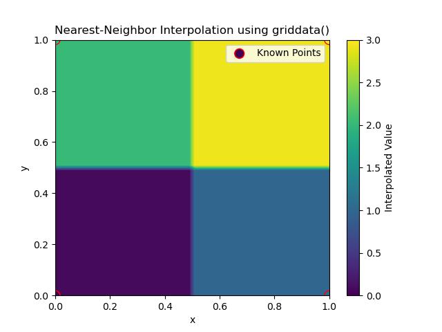
In this example the griddata() function is used to assign the values of the nearest points to all points on the grid. The plot shows how values are filled based on the nearest data point by creating blocky transitions −

import numpy as np
import matplotlib.pyplot as plt
from scipy.interpolate import griddata

# Define known data points and their values
points = np.array([[0, 0], [1, 0], [0, 1], [1, 1]])  # coordinates of known points
values = np.array([0, 1, 2, 3])  # function values at these points

# Create a grid of points where interpolation is needed
xi = np.linspace(0, 1, 50)
yi = np.linspace(0, 1, 50)
xi, yi = np.meshgrid(xi, yi)

# Perform Nearest-Neighbor Interpolation
zi = griddata(points, values, (xi, yi), method='nearest')

# Plot the interpolated result
plt.contourf(xi, yi, zi, levels=20, cmap='viridis')
plt.scatter(points[:, 0], points[:, 1], c=values, s=100, edgecolor='red', label='Known Points')
plt.colorbar(label='Interpolated Value')
plt.title('Nearest-Neighbor Interpolation using griddata()')
plt.xlabel('x')
plt.ylabel('y')
plt.legend()
plt.show()

Following is the output of Nearest Neighbor Method in Grid Data Interpolation −

Cubic Interpolation in griddata()

In SciPy's griddata() the Cubic Interpolation is a method used to interpolate data over a grid when the data points are scattered. Cubic interpolation generates smooth surfaces by fitting cubic polynomials to the data points. This method provides a higher degree of smoothness compared to linear interpolation and is especially useful when the dataset contains smooth variations.

Below are the key features of Cubic interpolation in griddata() −

• Smooth Surface: Cubic interpolation produces smooth, continuous surfaces by making it ideal for datasets that require smooth transitions.
• Higher Accuracy: It provides better accuracy compared to nearest-neighbor and linear interpolation methods when smoothness is a priority.
• 2D Only: This method is currently available for two-dimensional interpolation and cannot be applied to higher-dimensional data directly..

To use cubic interpolation in griddata() we should simply set the method argument to 'cubic' −

griddata(points, values, xi, method='cubic')

Example

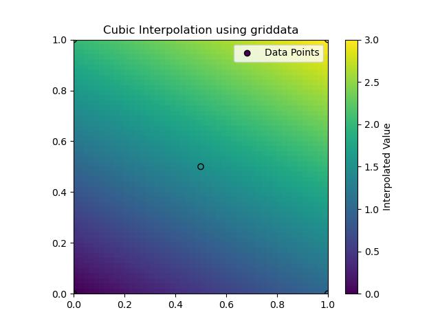
Following is the example which shows the usage of the method cubic in griddata() function of scipy −

import numpy as np
import matplotlib.pyplot as plt
from scipy.interpolate import griddata

# Define the known data points (coordinates)
points = np.array([[0, 0], [1, 0], [0, 1], [1, 1], [0.5, 0.5]])
values = np.array([0, 1, 2, 3, 1.5])  # The values at the known points

# Define the grid where interpolation will be performed
grid_x, grid_y = np.mgrid[0:1:50j, 0:1:50j]

# Perform cubic interpolation
grid_z = griddata(points, values, (grid_x, grid_y), method='cubic')

# Plot the result
plt.imshow(grid_z.T, extent=(0, 1, 0, 1), origin='lower', cmap='viridis')
plt.scatter(points[:, 0], points[:, 1], c=values, edgecolor='k', label='Data Points')
plt.title('Cubic Interpolation using griddata')
plt.colorbar(label='Interpolated Value')
plt.legend()
plt.show()

Following is the output of Cubic Method in Grid Data Interpolation −

Applications

Here are the applications of the Grid Data Mutli-dimensional Interpolation in scipy −

• Geographic Information Systems (GIS): Interpolating elevation or climate data over a geographic grid.
• Image Processing: Resampling and transforming pixel grids in images.
• Physics & Engineering: Interpolating sensor readings, temperature or pressure fields in simulations.
• Data Analysis: Filling in missing data points in multi-dimensional datasets.

Advantages

When we use the Grid Data Mutli-Dimensional Interpolation it posses the advantages, which are listed below −

• Flexibility: Works for scattered data points that are not regularly spaced.
• Multi-dimensional Support: Handles data of arbitrary dimensions by allowing it to be used in a variety of domains.
• Choice of Methods: Offers different interpolation methods to balance between computational efficiency and accuracy

Limitations

As we know when we use a particular method or process, it has the pro's as well as the con's. Here are the limitations of the Grid Data −

• Computational Cost: Cubic interpolation while smoother can be computationally expensive especially for large datasets.
• Boundary Extrapolation: For points outside the convex hull of the known data the results can be less reliable unless an appropriate fill_value is provided.

Finally we can conclude the SciPy's grid data multi-dimensional interpolation particularly via the griddata() function, is a powerful tool for estimating values in high-dimensional spaces where data may be sparse or irregularly spaced.

With multiple interpolation methods available the users can select the right approach based on the smoothness, accuracy and computational requirements of their specific problem.