SciPy - High Pass Filters

---

---

High Pass Filters

A High-pass Filter is used in image processing to emphasize the high-frequency components of an image such as edges, fine details and rapid intensity changes while suppressing the low-frequency components like smooth areas or gradual intensity variations. This makes high-pass filters especially useful for tasks like edge detection, image sharpening and feature enhancement.

Key concepts of High pass Filters

Following are the key concepts of High Pass Filters in SciPy −

• High Frequencies: These represent sharp intensity transitions such as edges, noise or fine textures.
• Low Frequencies: These represent smooth transitions such as uniform regions or gradual shading.
• Purpose: The purpose of these filters is to retain high-frequency details while attenuating low-frequency background information.

Types of High-Pass Filters

In High Pass Filters, we have different types and each filter is with its unique characteristics suited for specific tasks. They are −

• Gradient-Based Filters
• Sobel Filter
• Prewitt Filter
• Roberts Cross Filter
• Charr Filter
• Central Difference Filter

Let's go through the each filter in detail −

Spatial Domain High-Pass Filters

In image processing the spatial domain high-pass filters work by directly modifying pixel intensities to emphasize high-frequency components such as edges, fine details and rapid intensity transitions. These filters use convolution with specific kernels or operations to achieve the desired effect.

In spatial domain high-pass filters we have different types of filters which are as follows −

Gradient-Based Filters

Gradient-based filters are edge-detection techniques that emphasize intensity changes by calculating gradients i.e., first-order derivatives in an image. They are widely used in image processing for tasks like feature extraction, edge detection and object recognition.

The gradient of an image at a point is a vector representing the rate and direction of intensity changes where we can represent as magnitude (G) and Direction ().

• Magnitude(G): This indicates the strength of intensity change i.e., edge strength.

• Direction(): This represents the orientation of the edge.

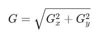
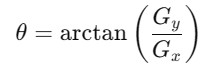
Where G_x and G_y are gradients in the horizontal and vertical directions, respectively.

In Gradient Filters, again we have different types which can be given as follows −

Sobel Filter

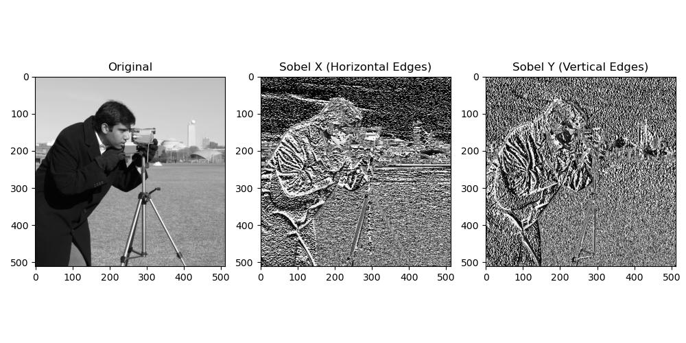
The Sobel filter is a gradient-based edge detection technique used in image processing to detect edges and highlight regions with high spatial frequency. It calculates the gradient of image intensity in the horizontal G_x and vertical G_y directions, which combines the results to produce an edge map.

In scipy, we have the scipy.ndimage.sobel() function to apply the sobel filter on the given image.

Syntax

Following is the syntax of using the scipy.ndimage.sobel() function to apply sobel filter on the image −

scipy.ndimage.sobel(input, axis=-1, output=None, mode='reflect', cval=0.0)

Following are the parameters of the scipy.ndimage.sobel() function −

• input (array_like): The input image or array on which the Sobel filter is applied and typically this is a 2d grayscale image.
• axis (int, optional): The axis along which to compute the derivative, when 1 applies the Sobel filter in the horizontal direction(G_x) and 0 applies the Sobel filter in the vertical direction(G_y)
• output (array or dtype, optional): This specifies where the output will be stored and if None then a new array is created and returned.
• mode (str, optional):: This defines how the input array is extended beyond its boundaries. The modes are such as reflect, constant, nearest, mirror and wrap.
• cval (scalar, optional): The constant value to use when mode='constant'. The default value is 0.0.

Following is the example of using the scipy.ndimage.sobel() function on the given image −

from scipy.ndimage import sobel
from skimage import data
import matplotlib.pyplot as plt

# Load a sample grayscale image
image = data.camera()

# Apply Sobel filter
sobel_x = sobel(image, axis=0)  # Horizontal edges
sobel_y = sobel(image, axis=1)  # Vertical edges
sobel_combined = sobel_x + sobel_y

# Display the results
plt.figure(figsize=(10, 5))
plt.subplot(1, 3, 1), plt.title("Original")
plt.imshow(image, cmap='gray')
plt.subplot(1, 3, 2), plt.title("Sobel X (Horizontal Edges)")
plt.imshow(sobel_x, cmap='gray')
plt.subplot(1, 3, 3), plt.title("Sobel Y (Vertical Edges)")
plt.imshow(sobel_y, cmap='gray')
plt.tight_layout()
plt.show()

Following is the output of the image on which the sobel filter is applied−

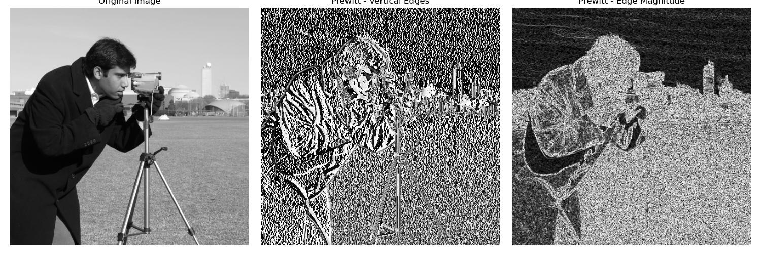
Prewitt Filter

The Prewitt filter is an edge detection operator used in image processing to highlight edges in an image by computing the gradient of pixel intensities. It is similar to the Sobel filter but uses different coefficients for its convolution masks. The Prewitt filter emphasizes the rate of intensity change in the horizontal and vertical directions.

This filter typically involves two convolution kernels (masks) used to calculate the gradients in the horizontal and vertical directions.

In scipy scipy.ndimage module does not have a built-in function for the Prewitt filter like the Sobel filter it is easy to implement using the convolve() function by directly applying the Prewitt kernels.

Following is the syntax of the function scipy.ndimage.convolve() used to apply the Prewitt filter −

scipy.ndimage.convolve(
   input, 
   weights, 
   output=None, 
   mode='reflect', 
   cval=0.0, 
   origin=0
)

Here are the parameters of the scipy.ndimage.convolve() function −

• input (array_like): The input image or array on which the convolution operation is applied. Typically this is a 2D grayscale image or a multidimensional array.
• weights (array_like): The filter or kernel to apply during the convolution. This should have the same number of dimensions as the input or be broadcastable.
• output (array or dtype, optional): This parameter specifies where the output will be stored. If None then a new array is created and returned.
• mode (str, optional): This parameter defines how the input array is extended beyond its boundaries. The available modes are such as 'reflect', 'constant', 'nearest', 'mirror' and 'wrap'. The default value is 'reflect'.
• cval (scalar, optional): The constant value used for padding when mode='constant'. The default value is 0.0.
• origin (int or tuple of ints, optional): This parameter controls the placement of the kernel relative to the input elements. Default value is 0 which centers the kernel.

Following is an example which uses the scipy.ndimage.convolve() function to apply the Prewitt filter to perform the edge detection in images both in horizontal and vertical edges based on intensity gradients −

import numpy as np
from scipy.ndimage import convolve
from skimage import data
import matplotlib.pyplot as plt

# Load a sample grayscale image
image = data.camera()

# Define Prewitt kernels for detecting vertical and horizontal edges
prewitt_vertical = np.array([[-1, 0, 1],
                             [-1, 0, 1],
                             [-1, 0, 1]])

prewitt_horizontal = np.array([[-1, -1, -1],
                               [ 0,  0,  0],
                               [ 1,  1,  1]])

# Apply the Prewitt filter in the vertical direction (horizontal edges)
edges_vertical = convolve(image, prewitt_vertical)

# Apply the Prewitt filter in the horizontal direction (vertical edges)
edges_horizontal = convolve(image, prewitt_horizontal)

# Combine the results by taking the magnitude of the gradient
edges_magnitude = np.sqrt(edges_vertical**2 + edges_horizontal**2)

# Display the results
plt.figure(figsize=(15, 5))

# Original Image
plt.subplot(1, 3, 1)
plt.title("Original Image")
plt.imshow(image, cmap='gray')
plt.axis('off')

# Vertical edges (horizontal gradient)
plt.subplot(1, 3, 2)
plt.title("Prewitt - Vertical Edges")
plt.imshow(edges_vertical, cmap='gray')
plt.axis('off')

# Magnitude of edges
plt.subplot(1, 3, 3)
plt.title("Prewitt - Edge Magnitude")
plt.imshow(edges_magnitude, cmap='gray')
plt.axis('off')

plt.tight_layout()
plt.show()

Following is the output of the convolve() function which is used to apply the prewitt filter −

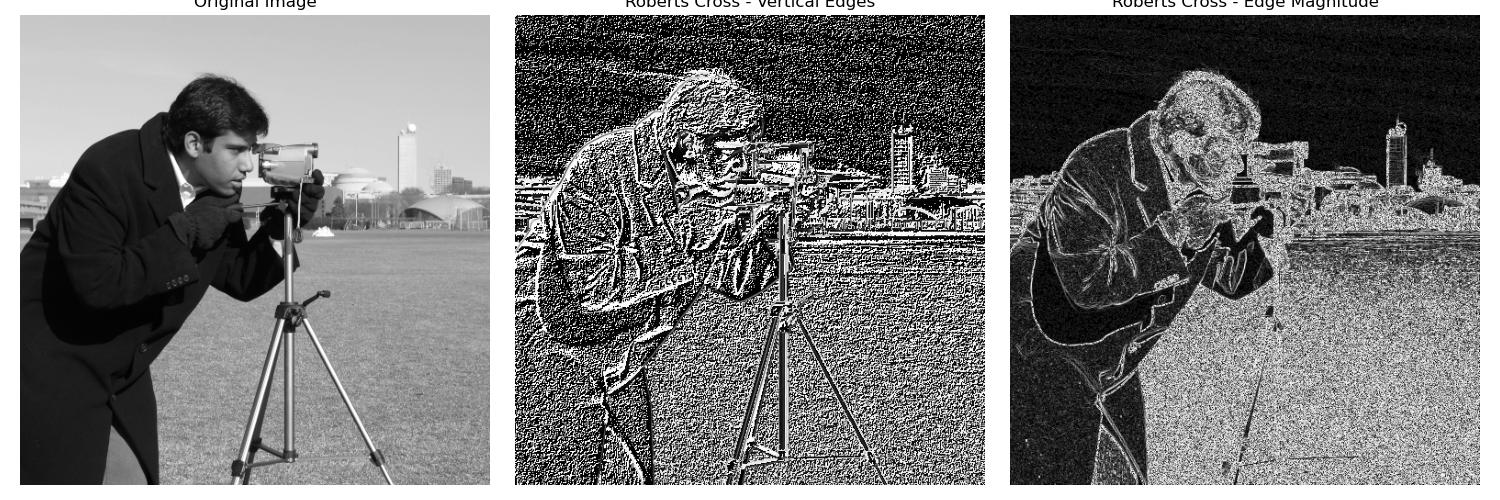
Roberts Cross Filter

The Roberts Cross filter is an edge detection operator used in image processing to highlight edges in an image by calculating the diagonal gradients of pixel intensities. It works by using small 2x2 convolution kernels by making it computationally efficient but sensitive to noise. The Roberts Cross filter emphasizes intensity changes along diagonals for detecting edges effectively in those directions.

This filter uses two convolution kernels (masks) to compute gradients in the diagonal directions.

In scipy.ndimage module we do not have a built-in function for the Roberts Cross filter. However it can be implemented using the convolve() function by directly applying the Roberts Cross kernels.

Following is an example which uses the scipy.ndimage.convolve() function to apply the Roberts Cross filter to detect edges in an image −

import numpy as np  
from scipy.ndimage import convolve  
from skimage import data  
import matplotlib.pyplot as plt  

# Load a sample grayscale image  
image = data.camera()  

# Define Roberts Cross kernels for diagonal gradients  
roberts_cross_vertical = np.array([[1, 0],  
                                    [0, -1]])  

roberts_cross_horizontal = np.array([[0, 1],  
                                      [-1, 0]])  

# Apply the Roberts Cross filter for diagonal gradients  
edges_vertical = convolve(image, roberts_cross_vertical)  
edges_horizontal = convolve(image, roberts_cross_horizontal)  

# Combine the results by taking the magnitude of the gradient  
edges_magnitude = np.sqrt(edges_vertical**2 + edges_horizontal**2)  

# Display the results  
plt.figure(figsize=(15, 5))  

# Original Image  
plt.subplot(1, 3, 1)  
plt.title("Original Image")  
plt.imshow(image, cmap='gray')  
plt.axis('off')  

# Vertical edges (horizontal gradient)  
plt.subplot(1, 3, 2)  
plt.title("Roberts Cross - Vertical Edges")  
plt.imshow(edges_vertical, cmap='gray')  
plt.axis('off')  

# Magnitude of edges  
plt.subplot(1, 3, 3)  
plt.title("Roberts Cross - Edge Magnitude")  
plt.imshow(edges_magnitude, cmap='gray')  
plt.axis('off')  

plt.tight_layout()  
plt.show()  

Following is the output of the convolve() function which is used to apply the Roberts Cross filter −

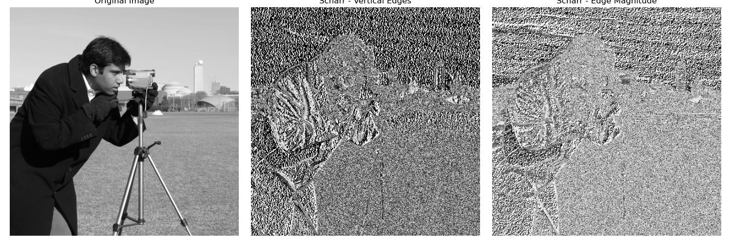
Scharr Filter

The Scharr filter is an edge detection operator used in image processing which is a variant of the Sobel filter designed to achieve better rotational symmetry and accuracy. It computes the gradient of pixel intensities in horizontal and vertical directions to highlight edges in an image. The Scharr filter is especially useful for applications requiring precise edge detection.

In SciPy we does not have any function to apply the scharr filter but we can implement it by using the scipy.ndimage.convolve(() function.

Following is an example that uses the scipy.ndimage.convolve() function to apply the Scharr filter and detect edges in an image −

import numpy as np 
from scipy.ndimage import convolve 
from skimage import data 
import matplotlib.pyplot as plt
#Load a sample grayscale image
image = data.camera()

#Define Scharr kernels for detecting vertical and horizontal edges
scharr_vertical = np.array([[-3, 0, 3],
[-10, 0, 10],
[-3, 0, 3]])

scharr_horizontal = np.array([[-3, -10, -3],
[0, 0, 0],
[3, 10, 3]])

#Apply the Scharr filter in the vertical direction (horizontal edges)
edges_vertical = convolve(image, scharr_vertical)

#Apply the Scharr filter in the horizontal direction (vertical edges)
edges_horizontal = convolve(image, scharr_horizontal)

#Combine the results by taking the magnitude of the gradient
edges_magnitude = np.sqrt(edges_vertical + edges_horizontal)

#Display the results
plt.figure(figsize=(15, 5))

#Original Image
plt.subplot(1, 3, 1)
plt.title("Original Image")
plt.imshow(image, cmap='gray')
plt.axis('off')

#Vertical edges (horizontal gradient)
plt.subplot(1, 3, 2)
plt.title("Scharr - Vertical Edges")
plt.imshow(edges_vertical, cmap='gray')
plt.axis('off')

#Magnitude of edges
plt.subplot(1, 3, 3)
plt.title("Scharr - Edge Magnitude")
plt.imshow(edges_magnitude, cmap='gray')
plt.axis('off')

plt.tight_layout()
plt.show()

Following is the output of the convolve() function used to apply the Scharr filter −

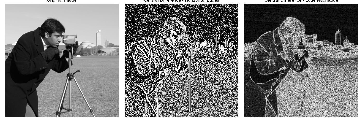
Central Difference Filter

The Central Difference filter is a gradient operator used in image processing to approximate the derivative of pixel intensities. It computes the difference between neighboring pixels symmetrically which helps detect changes in intensity by making it useful for edge detection tasks. This filter is simple and often used in applications where a basic gradient approximation is sufficient.

This filter uses a small convolution kernel to calculate gradients in the horizontal and vertical directions.

In scipy.ndimage the central difference filter can be implemented using the convolve() function by applying the appropriate central difference kernels.

Following is an example which uses the scipy.ndimage.convolve() function to apply the Central Difference filter to detect edges in an image −

import numpy as np  
from scipy.ndimage import convolve  
from skimage import data  
import matplotlib.pyplot as plt  

# Load a sample grayscale image  
image = data.camera()  

# Define Central Difference kernels for horizontal and vertical gradients  
central_diff_horizontal = np.array([[-1, 0, 1]])  
central_diff_vertical = np.array([[-1], [0], [1]])  

# Apply the Central Difference filter in the horizontal direction  
edges_horizontal = convolve(image, central_diff_horizontal)  

# Apply the Central Difference filter in the vertical direction  
edges_vertical = convolve(image, central_diff_vertical)  

# Combine the results by taking the magnitude of the gradient  
edges_magnitude = np.sqrt(edges_horizontal**2 + edges_vertical**2)  

# Display the results  
plt.figure(figsize=(15, 5))  

# Original Image  
plt.subplot(1, 3, 1)  
plt.title("Original Image")  
plt.imshow(image, cmap='gray')  
plt.axis('off')  

# Horizontal Edges  
plt.subplot(1, 3, 2)  
plt.title("Central Difference - Horizontal Edges")  
plt.imshow(edges_horizontal, cmap='gray')  
plt.axis('off')  

# Magnitude of Edges  
plt.subplot(1, 3, 3)  
plt.title("Central Difference - Edge Magnitude")  
plt.imshow(edges_magnitude, cmap='gray')  
plt.axis('off')  

plt.tight_layout()  
plt.show()  

Following is the output of the convolve() function which is used to apply the Central Difference filter −