SciPy - Image Transformation

---

---

SciPy's Image Transformation which is a functionality provides a set of tools for performing various transformations on images such as scaling, rotating, translating and warping. These operations are useful in applications such as image processing, computer vision and data augmentation for machine learning models.

SciPy uses its scipy.ndimage module to handle image transformations. This module is part of the broader SciPy library and is designed specifically for multidimensional image processing.

Key Features of Image Transformation in SciPy

Below are the key features that make SciPy's image transformation capabilities powerful and adaptable −

• Affine Transformations: This include operations such as scaling, rotating, shearing and translating an image while maintaining straight lines and parallelism. To perform this feature we can use the function scipy.ndimage.affine_transform().
• Geometric Transformations: These transformations involve remapping pixels using a mathematical function that specifies new pixel coordinates. These are useful for more general, custom transformations such as warping or bending the image and this can be achieved with the help of scipy.ndimage.affine_transform() function.
• Rotation: Rotating an image around a point by a specified angle can be achieved with this rotation feature. This feature supports interpolation for smoother rotations and the option to preserve or change the image shape i.e., bounding box. This can be achived with the help of scipy.ndimage.rotate()
• Zoom (Scaling): Scaling the image either uniformly or non-uniformly along each axis. This feature is mainly used for resizing images or performing zooming effects for images. To achieve this scaling we can use the function scipy.ndimage.zoom().
• Shifting (Translation): Translating (shifting) an image by a specified number of pixels along each axis. This feature is used for translating an image by arbitrary amounts without affecting its content. The scipy.ndimage.shift() function is used to perform shift operation.
• Warping: When applying a non-linear transformation that remaps the coordinates of an image to custom positions. This allows for more complex image distortions or adjustments. Here this is used for tasks such as perspective corrections or non-linear adjustments to the image. It uses the function scipy.ndimage.map_coordinates().
• Interpolation Methods: Different interpolation methods control how pixel values are estimated during transformations. The Interpolation methods are such as Nearest neighbor, Bilinear, Bicubic. Many transformation functions such as rotate, affine_transform, zoom allow users to select interpolation methods.
• Boundary Handling: It control how pixel values are handled at the edges of the image where transformation might go beyond the original boundaries. Here in this we have the different options such as constant, nearest, wrap and mirror. We can use parameter mode='constant' and mode='nearest' to perform this boundary handling.
• Custom Transformation Functions: Users can specify their own transformation functions to remap pixels in a customized manner. The function scipy.ndimage.geometric_transform() is used to perform Custom Transformation.
• Multi-dimensional Support: SciPy supports transformations not just for 2D images but also for higher-dimensional arrays such as 3D, 4D, etc by making it versatile for volumetric data and time-series data. All the above transformation functions work for n-dimensional arrays.

Let's see commonly used transformation techniques with examples in brief −

Rotation of Image

Rotation is a fundamental image transformation that turns an image around a specific point which is usually the center by a given angle. SciPy provides the scipy.ndimage.rotate() function for this purpose which is flexible and supports a range of options like interpolation and boundary handling.

Syntax

Following is the syntax of the function scipy.ndimage.rotate() −

scipy.ndimage.rotate(input, angle, axes=(1, 0), reshape=True, order=3, mode='constant', cval=0.0, prefilter=True)

Here are the parameters of the function scipy.ndimage.rotate() −

• input: The input array (image).
• angle: The rotation angle in degrees.
• axes: The axes defining the plane of rotation with default value as (1, 0) for 2D images.
• reshape: Whether to adjust the output shape to fit the rotated image.
• order: The interpolation order with the default value is 3 for cubic.
• mode: Boundary mode such as 'constant', 'reflect'.
• cval: Constant value to fill when mode = 'constant'.
• prefilter: Pre-filtering for higher-order interpolation i.e., usually left as True.

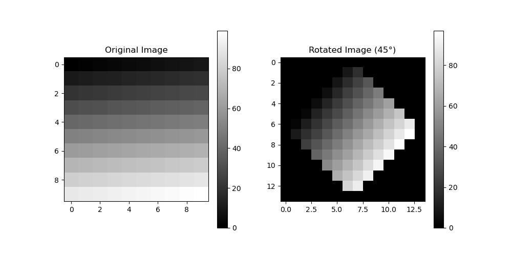
Following is the example to perform the rotation of the image with the help of scipy.ndimage.rotate() function −

import numpy as np
from scipy.ndimage import rotate
import matplotlib.pyplot as plt

# Create a simple 2D array as an image (gradient)
image = np.arange(100).reshape(10, 10)

# Rotate the image by 45 degrees
rotated_image = rotate(image, angle=45, reshape=True)

# Display the original and rotated images
plt.figure(figsize=(10, 5))
plt.subplot(1, 2, 1)
plt.title("Original Image")
plt.imshow(image, cmap='gray')
plt.colorbar()

plt.subplot(1, 2, 2)
plt.title("Rotated Image (45)")
plt.imshow(rotated_image, cmap='gray')
plt.colorbar()
plt.show()

Here is the output of the roatated image using the scipy.ndimage.rotate() function −

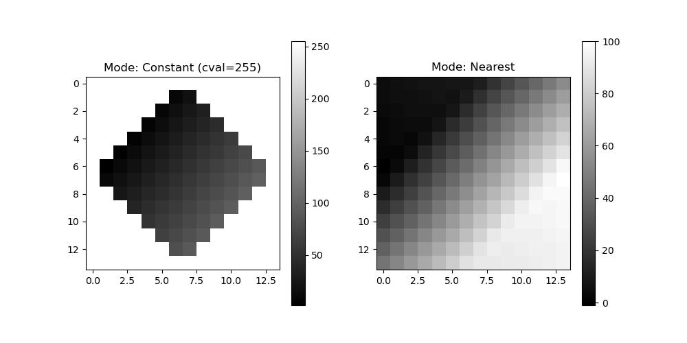
Here is another example which rotates the image by defining the boundary modes to the scipy.ndimage.rotate() function −

import numpy as np
from scipy.ndimage import rotate
import matplotlib.pyplot as plt

# Create a simple 2D array as an image (gradient)
image = np.arange(100).reshape(10, 10)

rotated_constant = rotate(image, angle=45, mode='constant', cval=255)
rotated_nearest = rotate(image, angle=45, mode='nearest')

plt.figure(figsize=(10, 5))
plt.subplot(1, 2, 1)
plt.title("Mode: Constant (cval=255)")
plt.imshow(rotated_constant, cmap='gray')
plt.colorbar()

plt.subplot(1, 2, 2)
plt.title("Mode: Nearest")
plt.imshow(rotated_nearest, cmap='gray')
plt.colorbar()

plt.show()

Here is the output of the roatated image using the scipy.ndimage.rotate() function within the defined boundaries −

Scaling an Image

Scaling is the process of resizing an image by increasing or decreasing its dimensions along one or more axes. SciPy provides the scipy.ndimage.zoom() function for this purpose which allows users to scale images with control over interpolation and boundary handling.

Syntax

Following is the syntax for using the scipy.ndimage.zoom() function to perform scaling on the image −

scipy.ndimage.zoom(input, zoom, order=3, mode='constant', cval=0.0, prefilter=True)

Here are the parameters of the function scipy.ndimage.rotate() −

• input: The input array (image).
• zoom: The zoom factor(s). A scalar or a sequence of factors for each axis.
• order: Interpolation order (default is 3 for cubic).
• mode:Boundary mode such as 'constant', 'reflect'.
• cval: Constant value to fill for mode='constant'.
• prefilter: Whether to prefilter the input for higher-order interpolation.

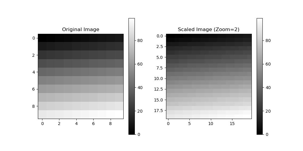
Following is an example which perform scaling to an image uniformly with the help of the function scipy.ndimage.zoom() −

import numpy as np
from scipy.ndimage import zoom
import matplotlib.pyplot as plt

# Create a simple 2D array (gradient image)
image = np.arange(100).reshape(10, 10)

# Scale the image by a factor of 2
scaled_image = zoom(image, zoom=2)

# Display the original and scaled images
plt.figure(figsize=(10, 5))
plt.subplot(1, 2, 1)
plt.title("Original Image")
plt.imshow(image, cmap='gray')
plt.colorbar()

plt.subplot(1, 2, 2)
plt.title("Scaled Image (Zoom=2)")
plt.imshow(scaled_image, cmap='gray')
plt.colorbar()

plt.show()

Here is the output of the image which had scaling uniformly −

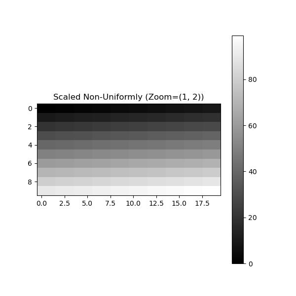
Here is the example of scaling an image with the non-uniform factors by using the function scipy.ndimage.zoom() −

import numpy as np
from scipy.ndimage import zoom
import matplotlib.pyplot as plt

# Create a simple 2D array as an image (gradient)
image = np.arange(100).reshape(10, 10)

# Scale with different factors for each axis
scaled_non_uniform = zoom(image, zoom=(1, 2))  # Scale rows by 1, columns by 2

plt.figure(figsize=(6, 6))
plt.title("Scaled Non-Uniformly (Zoom=(1, 2))")
plt.imshow(scaled_non_uniform, cmap='gray')
plt.colorbar()
plt.show()

Here is the output of the image scaled with non uniform factors −

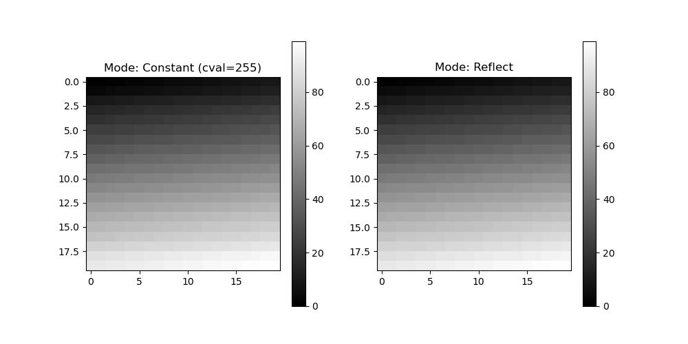
Below is another example which specifies the boundaries to the function scipy.ndimage.zoom() to perform the scaling on the image −

import numpy as np
from scipy.ndimage import zoom
import matplotlib.pyplot as plt

# Create a simple 2D array as an image (gradient)
image = np.arange(100).reshape(10, 10)

scaled_constant = zoom(image, zoom=2, mode='constant', cval=255)
scaled_reflect = zoom(image, zoom=2, mode='reflect')

plt.figure(figsize=(10, 5))
plt.subplot(1, 2, 1)
plt.title("Mode: Constant (cval=255)")
plt.imshow(scaled_constant, cmap='gray')
plt.colorbar()

plt.subplot(1, 2, 2)
plt.title("Mode: Reflect")
plt.imshow(scaled_reflect, cmap='gray')
plt.colorbar()

plt.show()

Here is the output of the scaling image within specified boundary modes −

Translation of Image

Translation refers to shifting an image by a specified distance along one or more axes. SciPy provides the scipy.ndimage.shift() function for performing translation operations on images or multidimensional arrays. This can be useful for image augmentation, alignment or spatial transformations.

Syntax

Here is the syntax for using the scipy.ndimage.shift() function to perform the image translation −

scipy.ndimage.shift(input, shift, order=3, mode='constant', cval=0.0, prefilter=True)

Here are the parameters of the function scipy.ndimage.shift() −

• input: The input array (image).
• shift: The shift values, specified as a scalar or a sequence of shifts for each axis.
• order: Interpolation order with the default value 3 for cubic).
• mode: Boundary mode such as 'constant', 'reflect', 'nearest' or 'wrap'.
• cval: Constant value to fill for mode='constant'.
• prefilter: Whether to prefilter the input for higher-order interpolation.

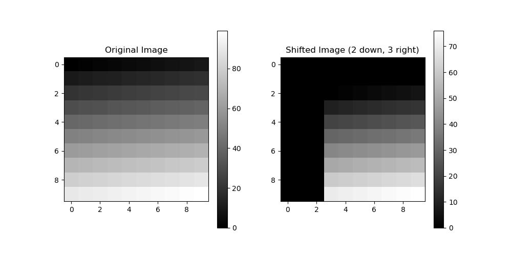
Here is the example which performs the basic translation of the image by using the function scipy.ndimage.shift() −

import numpy as np
from scipy.ndimage import shift
import matplotlib.pyplot as plt

# Create a simple 2D array (gradient image)
image = np.arange(100).reshape(10, 10)

# Translate the image by 2 pixels down and 3 pixels to the right
shifted_image = shift(image, shift=(2, 3))

# Display the original and shifted images
plt.figure(figsize=(10, 5))
plt.subplot(1, 2, 1)
plt.title("Original Image")
plt.imshow(image, cmap='gray')
plt.colorbar()

plt.subplot(1, 2, 2)
plt.title("Shifted Image (2 down, 3 right)")
plt.imshow(shifted_image, cmap='gray')
plt.colorbar()

plt.show()

Here is the output of the simple image translation with the help of scipy.ndimage.shift() function −

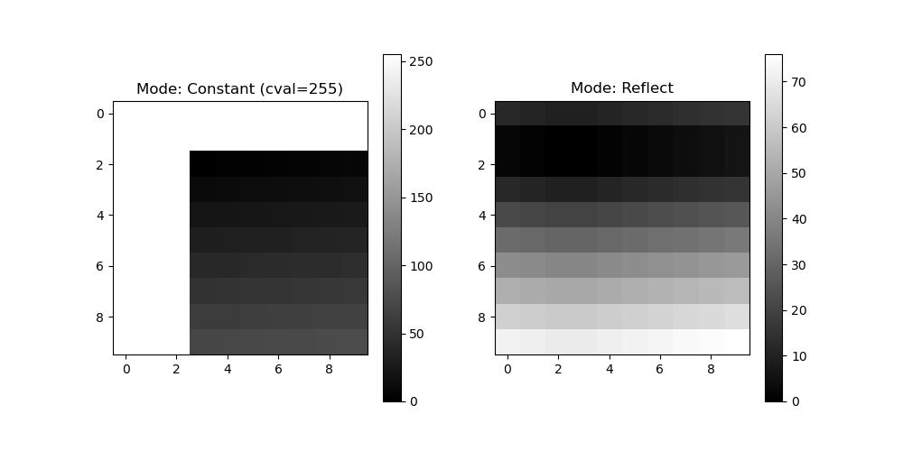
Following is another example which performs the image translation within the specified boundary modes passed to the scipy.ndimage.shift() function −

import numpy as np
from scipy.ndimage import shift
import matplotlib.pyplot as plt

# Create a simple 2D array (gradient image)
image = np.arange(100).reshape(10, 10)

# Translate with constant boundary (fill with 255)
shifted_constant = shift(image, shift=(2, 3), mode='constant', cval=255)

# Translate with reflect boundary mode
shifted_reflect = shift(image, shift=(2, 3), mode='reflect')

plt.figure(figsize=(10, 5))
plt.subplot(1, 2, 1)
plt.title("Mode: Constant (cval=255)")
plt.imshow(shifted_constant, cmap='gray')
plt.colorbar()

plt.subplot(1, 2, 2)
plt.title("Mode: Reflect")
plt.imshow(shifted_reflect, cmap='gray')
plt.colorbar()

plt.show()

Here is the output of the image in which translation was done within the specified boundary modes using the scipy.ndimage.shift() function −

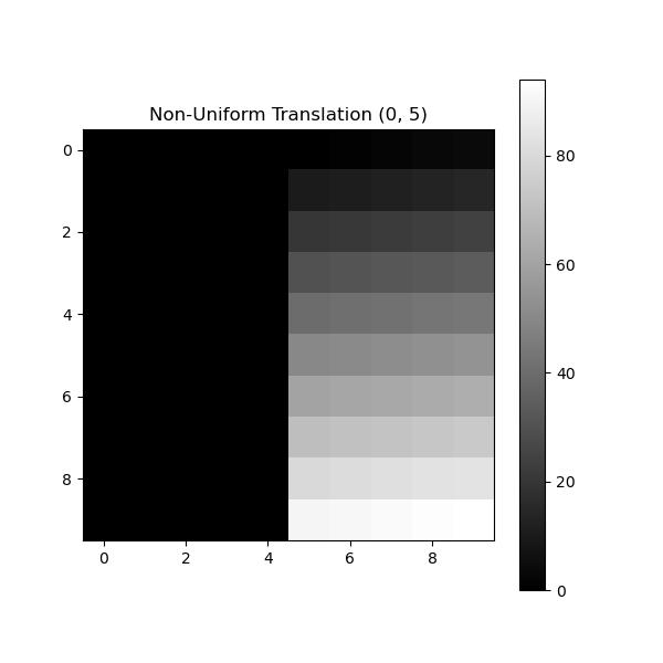
Here is the example of performing Non - uniform translation −

import numpy as np
from scipy.ndimage import shift
import matplotlib.pyplot as plt

# Create a simple 2D array (gradient image)
image = np.arange(100).reshape(10, 10)

# Shift by different amounts along rows and columns
shifted_non_uniform = shift(image, shift=(0, 5))  # No vertical shift, 5-pixel horizontal shift

plt.figure(figsize=(6, 6))
plt.title("Non-Uniform Translation (0, 5)")
plt.imshow(shifted_non_uniform, cmap='gray')
plt.colorbar()
plt.show()

Here is the output of the image with non uniform translation −

Affine Transformations

Affine transformations are a class of geometric transformations that preserve points, straight lines and planes. They can involve operations such as translation, rotation, scaling and shearing while maintaining the basic structure of the image such as parallel lines remain parallel and ratios of distances are preserved. In SciPy affine transformations can be performed using the scipy.ndimage.affine_transform() function.

Syntax

Following is the syntax for using the scipy.ndimage.affine_transform() function to perform the geometric transformations −

scipy.ndimage.affine_transform(input, matrix, offset=0, output_shape=None, order=3, mode='constant', cval=0.0, prefilter=True)

Here are the parameters of the function scipy.ndimage.affine_transform() −

• input: The input array (image).
• matrix: The linear transformation matrix which is typically a 2x2 matrix for 2D images or 3x3 for 3D images.
• offset: The translation vector specify the amount to shift the image after applying the matrix transformation.
• output_shape: The shape of the output array. If not specified then it is inferred from the input.
• order: Interpolation order with the default value 3 for cubic interpolation.
• mode: Boundary mode such as 'constant', 'reflect', 'nearest' or 'wrap'.
• cval: Constant value to fill for mode='constant'.
• prefilter: Whether to prefilter the input for higher-order interpolation.

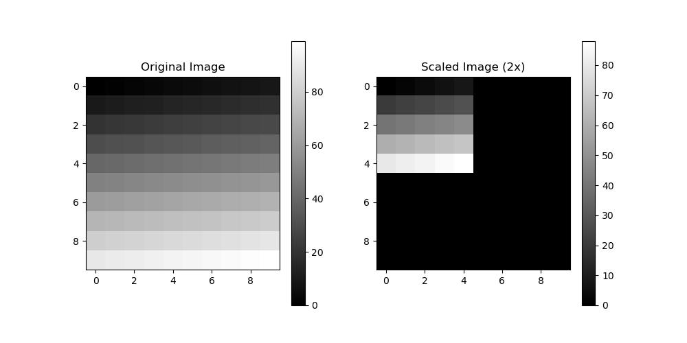
Here is the example of simple Affine transformation which performs scaling and translation of the image together by using the function scipy.ndimage.affine_transform() −

import numpy as np
from scipy.ndimage import affine_transform
import matplotlib.pyplot as plt

# Create a simple 2D image (gradient)
image = np.arange(100).reshape(10, 10)

# Define a scaling matrix (scale by 2 in x and y)
matrix = np.array([[2, 0], [0, 2]])  # Scaling by 2 in both axes
offset = [0, 0]  # No translation

# Apply affine transformation (scaling)
scaled_image = affine_transform(image, matrix, offset=offset, order=1)

# Display original and scaled image
plt.figure(figsize=(10, 5))
plt.subplot(1, 2, 1)
plt.title("Original Image")
plt.imshow(image, cmap='gray')
plt.colorbar()

plt.subplot(1, 2, 2)
plt.title("Scaled Image (2x)")
plt.imshow(scaled_image, cmap='gray')
plt.colorbar()

plt.show()

Here is the output of the simple affline transformation using the scipy.ndimage.affline_transform() function −

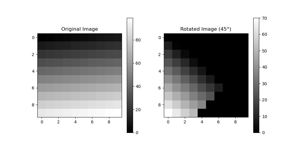
Following is the example which performs the Affine Transformation with Rotation and Translation using the function scipy.ndimage.affine_transform() −

import numpy as np
from scipy.ndimage import affine_transform
import matplotlib.pyplot as plt

# Create a simple 2D image (gradient)
image = np.arange(100).reshape(10, 10)

# Define a scaling matrix (scale by 2 in x and y)
matrix = np.array([[2, 0], [0, 2]])  # Scaling by 2 in both axes
offset = [0, 0]  # No translation

# Define a rotation matrix (rotate by 45 degrees)
theta = np.radians(45)  # Convert to radians
rotation_matrix = np.array([[np.cos(theta), -np.sin(theta)], [np.sin(theta), np.cos(theta)]])
offset = [0, 0]  # No translation

# Apply affine transformation (rotation)
rotated_image = affine_transform(image, rotation_matrix, offset=offset, order=1)

# Display original and rotated image
plt.figure(figsize=(10, 5))
plt.subplot(1, 2, 1)
plt.title("Original Image")
plt.imshow(image, cmap='gray')
plt.colorbar()

plt.subplot(1, 2, 2)
plt.title("Rotated Image (45)")
plt.imshow(rotated_image, cmap='gray')
plt.colorbar()

plt.show()

Here is the output of the affline transformation along with rotation and translation using the scipy.ndimage.affline_transform() function −

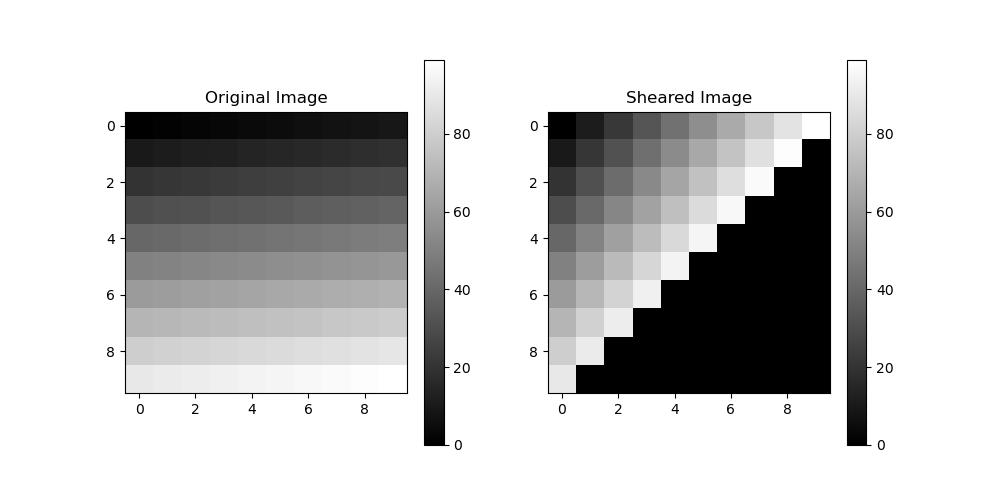
In this example we will perform the Affline Transformation with shearing by using the function scipy.ndimage.affine_transform() −

import numpy as np
from scipy.ndimage import affine_transform
import matplotlib.pyplot as plt

# Create a simple 2D image (gradient)
image = np.arange(100).reshape(10, 10)

# Define a scaling matrix (scale by 2 in x and y)
matrix = np.array([[2, 0], [0, 2]])  # Scaling by 2 in both axes
offset = [0, 0]  # No translation

# Define a shearing matrix (shear along x-axis)
shear_matrix = np.array([[1, 1], [0, 1]])  # Shear along x-axis
offset = [0, 0]  # No translation

# Apply affine transformation (shearing)
sheared_image = affine_transform(image, shear_matrix, offset=offset, order=1)

# Display original and sheared image
plt.figure(figsize=(10, 5))
plt.subplot(1, 2, 1)
plt.title("Original Image")
plt.imshow(image, cmap='gray')
plt.colorbar()

plt.subplot(1, 2, 2)
plt.title("Sheared Image")
plt.imshow(sheared_image, cmap='gray')
plt.colorbar()

plt.show()

Following is the output of the affline transformation which performs shearing of the image with the help of scipy.ndimage.affline_transform() function −