SciPy - Integration of Ordinary Differential Equations (ODEs)

---

---

In SciPy the integration of Ordinary Differential Equations(ODEs) is handled using the solve_ivp() function which provides a versatile way to solve initial value problems (IVPs) for ODEs.

This function integrates systems of first-order ODEs or higher-order ODEs that have been reduced to first-order form. The general structure of an ODE problem is given as follows −

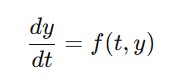
Where y is the state variable(s), t is the independent variable (often time) and f(t,y) defines the system dynamics.

When we want to use solve_ivp() function we have to specify the ODE system, the time span over which to integrate, the initial conditions and optional parameters such as the method RK45, BDF for stiff problems. This function outputs a solution object containing the time points, state variables and whether the integration was successful.

Integration methods for ODEs include both analytical and numerical approaches. Analytical methods such as separation of variables or integrating factors are aimed to find an exact solution in the form of a closed expression.

However many ODEs cannot be solved analytically by requiring numerical methods such as Euler's method, Runge-Kutta methods or adaptive step-size algorithms. These techniques approximate the solution by discretizing the problem and iterating over small intervals.

Ordinary Differential Equations(ODEs) are crucial in modeling dynamic systems in physics, biology, economics and engineering where they describe phenomena such as motion, population growth or chemical reactions. The integration process helps predict system behavior over time by solving for the dependent variable.

Key Concepts in ODEs

Here are the characteristics that help us to classify ODEs and determine the appropriate solution techniques −

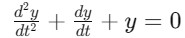
• Order: The order of an ODE is defined by the highest derivative in the equation. For instance let's consider the equation in which is a second-order ODE because the highest derivative is the second derivative.

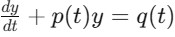
• Linear vs Nonlinear: A linear ODE general form is given as follows, where y and its derivatives appear only to the first power.−

  

  A nonlinear ODE involves powers or products of y or its derivatives which is given as follows −

  
• Homogeneous vs Nonhomogeneous: A homogeneous ODE contains only terms involving y or its derivatives i.e., f(t,y)=0 where a nonhomogeneous ODE includes an additional function such as dy/dt = y+g(t).
• Initial Value Problem (IVP): In an IVP the function's value at a starting time is specified and the solution is found from that initial condition.
• Boundary Value Problem (BVP): In a BVP the solution is sought over a specific range with conditions provided at the boundaries instead of just one initial point.
• Stiffness: ODEs with rapidly changing solutions are called stiff and often need implicit solvers such as BDF for efficient solution.

The solve_ivp() function in scipy.integrate Module

solve_ivp() is a versatile function in SciPys scipy.integrate module for solving initial value problems (IVP) for systems of ordinary differential equations (ODEs). It supports multiple integration methods such as RK45, RK23 and BDF for adapting step sizes based on error estimates for efficiency.

Syntax

Following is the syntax of solve_ivp() function of scipy.integrate module to perform integration of ordinary differential Equations −

scipy.integrate.solve_ivp(fun, t_span, y0, method='RK45', t_eval=None, dense_output=False, events=None, vectorized=False, args=None, **options)

Parameters

Here are the parameters of the scipy.integrate.solve_ivp() function −

• fun: A callable function that defines the system of ODEs. It takes two arguments namely, time 't' and state variable 'y'.
• t_span: A tuple (t0, tf) representing the interval of integration from the initial time (t₀,t_f) to the final time t_f.
• y0: Initial conditions at t₀ for the system of ODEs. It can be a scalar or an array.
• method: Specifies the integration method. Default is 'RK45' an explicit Runge-Kutta method. Other methods include 'RK23', 'BDF' (for stiff problems) and 'DOP853'.
• t_eval(optional): An array of time points where the solution is desired. If not provided the solver chooses its own time points.
• dense_output(optional):If True then enables interpolation of the solution between time points via a continuous solution. Default value is False.
• events(optional) A function or list of functions to detect events for example when a specific condition is met such as crossing a threshold. The solver stops integration when an event is triggered.
• vectorized(optional): Set to True if fun(t, y) is vectorized which means it can process arrays of y values simultaneously.
• args(optional): Additional arguments passed to the ODE function fun.
• **options: Extra options for specific methods such as step size control or error tolerance.

Example 1

Following is the example of using the scipy.integrate.solve_ivp() function for calculating the integration of ordinary differential equations −

from scipy.integrate import solve_ivp
import numpy as np

# Define the ODE system
def fun(t, y):
    return -0.5 * y

# Time span and initial condition
t_span = (0, 10)
y0 = [2]

# Solve ODE
sol = solve_ivp(fun, t_span, y0, method='RK45', t_eval=np.linspace(0, 10, 100))

# Access the solution
print(sol.t)  # Time points
print(sol.y)  # Solution values at the time points

Here is the output of using the solve_ivp() function of scipy.integrate module −

[ 0.          0.1010101   0.2020202   0.3030303   0.4040404   0.50505051
  0.60606061  0.70707071  0.80808081  0.90909091  1.01010101  1.11111111
  1.21212121  1.31313131  1.41414141  1.51515152  1.61616162  1.71717172
  1.81818182  1.91919192  2.02020202  2.12121212  2.22222222  2.32323232
  2.42424242  2.52525253  2.62626263  2.72727273  2.82828283  2.92929293
  ----------------------------------------------------------------------
  ----------------------------------------------------------------------
  ----------------------------------------------------------------------
   0.038976   0.03706282 0.03524353 0.03351272 0.03186515 0.03029604
  0.02880286 0.02738259 0.02603204 0.02474807 0.02352765 0.02236783
  0.02126571 0.02021851 0.01922349 0.01827802 0.01737954 0.01652556
  0.01571368 0.01494158 0.01420701 0.01350782]]

Example 2

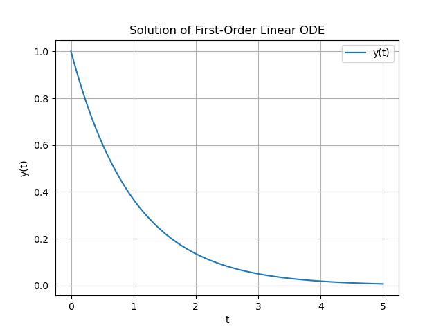
Here is an example of solving a first-order linear ODE using SciPy's solve_ivp function then the solution y(t) is the numerical solution to the ODE, plotted for t in the range [0, 5] −

import numpy as np
from scipy.integrate import solve_ivp
import matplotlib.pyplot as plt

# Define the ODE as a function
def linear_ode(t, y):
    return np.exp(-t) - 2 * y

# Time span and initial condition
t_span = (0, 5)
y0 = [1]

# Time points where the solution is computed
t_eval = np.linspace(0, 5, 100)

# Solve the ODE
sol = solve_ivp(linear_ode, t_span, y0, method='RK45', t_eval=t_eval)

# Plot the solution
plt.plot(sol.t, sol.y[0], label='y(t)')
plt.xlabel('t')
plt.ylabel('y(t)')
plt.title('Solution of First-Order Linear ODE')
plt.grid()
plt.legend()
plt.show()

Here is the output of the first order ODE using the solve_ivp() function −

Example 3

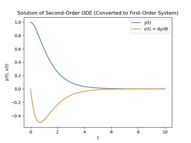
A second-order ODE can be converted into a system of first-order ODEs to solve numerically using SciPys solve_ivp. The key idea is to reduce the second-order ODE into two coupled first-order equations −

import numpy as np
from scipy.integrate import solve_ivp
import matplotlib.pyplot as plt

# Define the system of first-order ODEs
def system(t, Y):
    y, v = Y  # Y is a vector containing [y, v]
    dydt = v  # First equation: dy/dt = v
    dvdt = -3*v - 2*y  # Second equation: dv/dt = -3v - 2y
    return [dydt, dvdt]

# Time span and initial conditions
t_span = (0, 10)
y0 = [1, 0]  # Initial conditions: y(0) = 1, v(0) = dy/dt(0) = 0

# Solve the system
sol = solve_ivp(system, t_span, y0, t_eval=np.linspace(0, 10, 100))

# Plot the solution
plt.plot(sol.t, sol.y[0], label='y(t)')  # y(t)
plt.plot(sol.t, sol.y[1], label="v(t) = dy/dt")  # v(t)
plt.xlabel('t')
plt.ylabel('y(t), v(t)')
plt.legend()
plt.title('Solution of Second-Order ODE (Converted to First-Order System)')
plt.show()

Here is the output of the first order ODE using the solve_ivp() function −

Example 4

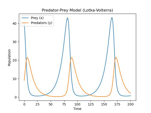
The Predator-Prey Model is a well-known example of coupled ODEs that describes the interaction between two species namely, predators and prey. The model is often referred to as the Lotka-Volterra equations. Here is the example of it −

import numpy as np
from scipy.integrate import solve_ivp
import matplotlib.pyplot as plt

# Define the system of equations (Predator-Prey Model)
def predator_prey(t, z, alpha, beta, delta, gamma):
    x, y = z  # z is a vector containing [x, y]
    dxdt = alpha * x - beta * x * y  # Prey equation
    dydt = delta * x * y - gamma * y  # Predator equation
    return [dxdt, dydt]

# Parameters
alpha = 0.1  # Prey growth rate
beta = 0.02  # Predation rate
delta = 0.01  # Predator reproduction rate
gamma = 0.1  # Predator death rate

# Time span and initial conditions
t_span = (0, 200)
y0 = [40, 9]  # Initial populations: 40 prey, 9 predators

# Solve the system of equations
sol = solve_ivp(predator_prey, t_span, y0, args=(alpha, beta, delta, gamma), 
                t_eval=np.linspace(0, 200, 1000))

# Plot the results
plt.plot(sol.t, sol.y[0], label='Prey (x)')
plt.plot(sol.t, sol.y[1], label='Predators (y)')
plt.xlabel('Time')
plt.ylabel('Population')
plt.title('Predator-Prey Model (Lotka-Volterra)')
plt.legend()
plt.show()

Following is the output of the above example −