SciPy - Integration of Stochastic Differential Equations

---

---

---

The Integration of Stochastic Differential Equations (SDEs) in SciPy is the process of solving differential equations that describe systems influenced by both deterministic and random components.

These equations are used to model various phenomena where uncertainty or noise is a fundamental characteristic, such as in finance, physics, biology and engineering.

Mathematically the Stochastic Differential Equations (SDEs) can be given as follows −

dXt = f(Xt,t)dt + g(Xt,t)dWt

Where −

• X_t is the state variable.
• f(X_t,t) represents the drift term i.e. deterministic part.
• g(X_t,t) is the diffusion term i.e. stochastic part.
• g(X_t,t) is the diffusion term i.e. stochastic part.
• W_t is a Wiener process or Brownian motion.
• dt is a small time increment.

Key Components of SDEs

Following are the key components of the Stochastic Differential Equations(SDEs) −

• Stochastic Process: A stochastic process introduces randomness into the system which often represented by Brownian motion, also called Wiener process. Brownian motion is a continuous-time random process characterized by unpredictable, continuous fluctuations.
• Drift Term: The deterministic part of an SDE which often denoted as f(X_t,t) represents the expected or average behavior of the system over time. This is similar to the rate of change in ordinary differential equations (ODEs).
• Diffusion Term: The stochastic part f(X_t,t) modulates the randomness in the system. This term is multiplied by the differential of Brownian motion dW_t which represents the random shocks that occur in the system.

Brownian Motion and Wiener Process

Brownian Motion and the Wiener Process are foundational concepts in the study of stochastic processes and are crucial for modeling randomness in various scientific fields such as finance, physics and engineering. Let's see about these in detail −

Brownian motion is also know as Wiener Process which describes the random movement of particles suspended in a fluid which was first observed by the botanist Robert Brown. Mathematically it has been formalized to represent continuous-time stochastic processes.

Following are the key properties of brownian motion −

• Start at Zero: Brownian motion starts at zero, i.e.,

  B(0) = 0
  

  This property establishes the starting point for the process and provides a reference for subsequent movement.

• Independent Increments: The increments of Brownian motion over non-overlapping intervals are independent.

  B(t+s)-B(t)
  

  It is independent of any past values B(u) for u < t which means that the future movement does not depend on the past trajectory of the process.

• Normally Distributed Increments: The increments of Brownian motion are normally distributed. Specifically for any value s > 0.

  B(t+s)-B(t)N(0,s)
  

  This indicates that the difference between the values of Brownian motion at two times t and t+s follows a normal distribution with a mean of 0 and variance equal to the length of the time interval s.

• Continuous Paths: The paths of Brownian motion are continuous which means that as time progresses, the function describing the motion does not have any jumps or discontinuities. However these paths are almost surely nowhere differentiable which signifies that they exhibit highly erratic behavior and cannot be described by a smooth function.

The mathematical representation of Brownian motion can be given as follows −

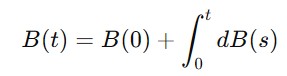
where B(0)=0 and dB(s) represents the infinitesimal increment of the Brownian motion.

Example

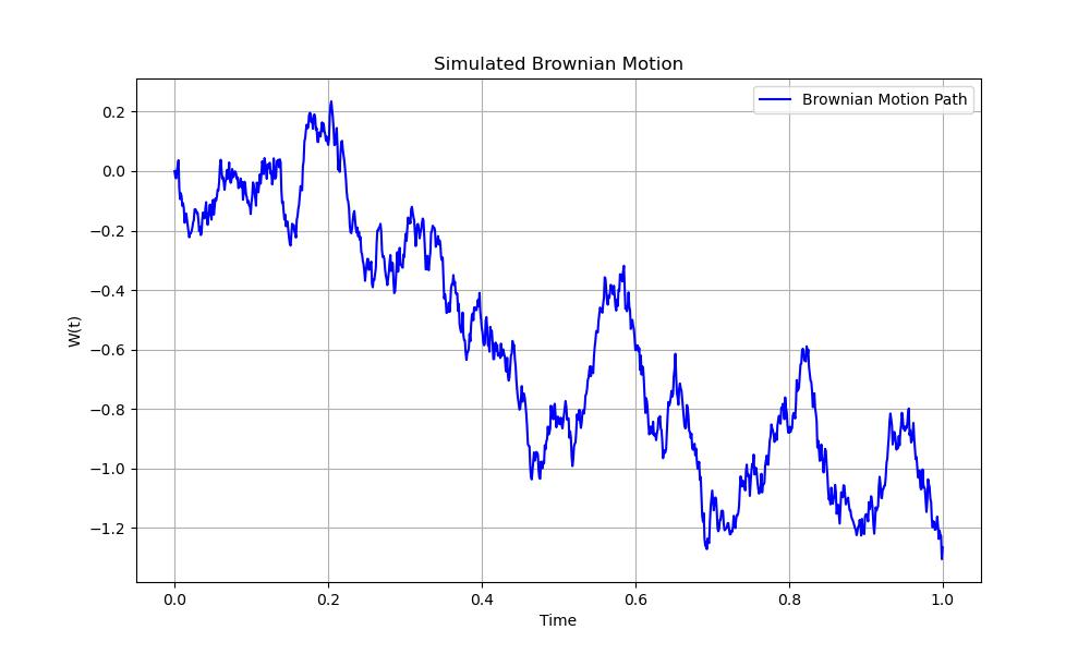
Below is an example that shows how to generate and plot a simple Brownian motion path using SciPy and Matplotlib −

import numpy as np
import matplotlib.pyplot as plt
from scipy.stats import norm

# Parameters
T = 1.0          # Total time
N = 1000        # Number of steps
dt = T/N        # Time increment
t = np.linspace(0, T, N+1)  # Time array

# Generate increments of the Wiener process
# dW is normally distributed with mean 0 and variance dt
dW = norm.rvs(loc=0.0, scale=np.sqrt(dt), size=N)  # Using scipy to generate normal increments
# Create the Brownian motion path by taking the cumulative sum of the increments
W = np.concatenate(([0], np.cumsum(dW)))

# Plotting the Brownian motion
plt.figure(figsize=(10, 6))
plt.plot(t, W, label='Brownian Motion Path', color='blue')
plt.title('Simulated Brownian Motion')
plt.xlabel('Time')
plt.ylabel('W(t)')
plt.grid()
plt.legend()
plt.show()

Following is the output of the Brownian motion −

Differences from Ordinary Differential Equations (ODEs)

In Ordinary Differential Equations (ODEs) the system evolves deterministically which means future states depend only on current values and time. However SDEs account for random influences by making the evolution of the system uncertain. This introduces more complexity in solving SDEs because the solutions are not deterministic paths but probability distributions over possible paths.

Integration of SDEs

The traditional methods used for integrating ODEs do not directly apply to SDEs due to the random component. There are specialized numerical techniques which are mentioned as below −

Euler-Maruyama Method

This is a simple and first-order numerical approximation technique for solving SDEs. It generalizes the Euler method for ODEs by including a random term.

For an SDE of the form

dXt = f(Xt,t)dt + g(Xt,t)dWt

which is Euler-Maruyama method approximates the solution as mentioned below −

Xt+tXt+f(Xt,t)t+g(Xt,t)tWt

Where, W_tN(0,_t)represents a random normal variable scaled by _t.

Milstein Method

This method is an enhancement over the Euler-Maruyama method it improves accuracy by accounting for the derivative of the diffusion term.

The Milstein method for an SDE is given as follows −

where g(X_t,t) is the derivative of the diffusion term with respect to X_t.

Applications of SDEs

Below are the applications of the Stochastic Differential Equations (SDEs) which are used in many fields to model systems where randomness plays a key role −

• Finance: In modeling stock prices such as Black-Scholes model for option pricing.
• Physics: For systems influenced by thermal noise such as particle motion in fluids.
• Biology: In population dynamics where birth and death processes involve randomness.
• Control Theory: For systems with random disturbances affecting control inputs.