SciPy - K Means Clustering

---

---

What is K-Means Clustering?

SciPy K-means clustering is a technique for partitioning data into 'K' clusters implemented in the scipy.cluster.vq module. It includes functions like 'kmeans' for clustering and 'vq' for assigning data points to clusters.

The algorithm works by iteratively updating cluster centroids and reassigning data points based on their distance to these centroids by aiming to minimize the within-cluster variance. SciPy's implementation allows for different initialization methods such as random or K-Means++ which improves centroid placement.

This clustering is useful for identifying groupings in datasets which although it is less feature-rich compared to other libraries such as scikit-learn.

Types of K-Means Clustering

K-means clustering is a widely used algorithm for partitioning data into clusters. Various types and variations of K-means clustering are employed to address specific needs or improve performance. Let's see them in detail −

Standard K-Means Clustering

Standard K-Means Clustering is a popular algorithm used for partitioning data into K distinct clusters. It works through an iterative process to assign data points to clusters and update cluster centroids.

How Does K-Means Clustering Work?

Here are the steps which shows how does the Standard K-Means Clustering works −

Initialization

Initialization is a crucial step in K-means clustering as it significantly impacts the algorithms performance and the quality of the final clustering results.

• Select the Number of Clusters (K) − Here we will decide the number of clusters that we want to form in the dataset. This is a crucial parameter that affects the results. We can use the methods such as Elbow, Silhouette Score, Gap Statistic, Cross-Validation as per our requiremnet.
• Initialize Centroids− We can start by randomly selecting (K) data points from our dataset to serve as the initial centroids (cluster centers). Alternatively, more advanced initialization methods such as K-Means++ can be employed to achieve better clustering results.

Assignment Step

The Assignment Step in K-means clustering is the phase where each data point in the dataset is assigned to the nearest cluster is based on the current positions of the centroids. This step is crucial because it determines the composition of each cluster which directly influencing the subsequent update step.

• Compute Distances − For each data point we calculate the distance to each of the K centroids. Common distance metrics such as Euclidean distance, Manhattan distance, etc.
• Assign Clusters− Assign each data point to the cluster associated with the nearest centroid. This forms K clusters where each data point belongs to the cluster with the closest centroid.

Update Step

The Update Step in the K-means clustering algorithm is crucial for refining the positions of the centroids based on the current cluster assignments of the data points. After the data points have been assigned to the nearest centroid i.e calculated in assignment step, the centroids are updated to reflect the mean position of all data points assigned to each cluster. This process continues iteratively until the centroids stabilize.

• Recalculate Centroids − Once all data points are assigned to clusters we can recompute the centroids for each cluster. The new centroid is calculated as the mean of all the data points within that cluster. Mathematically the formula is given as follows −

• Update Centroids − Replace the old centroids with the newly recalculated centroids.

• Convergence Check − After updating the centroids the algorithm checks whether the centroids have moved significantly compared to their previous positions.

  If the movement or change of centroids is below a certain threshold then the algorithm considers this as convergence and stops the iterations. Otherwise, the algorithm goes back to the Assignment Step to reassign data points to the nearest updated centroid.

Example

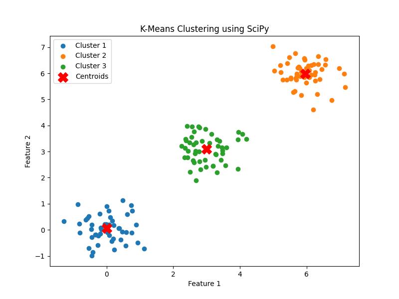
Following is the example which shows how to apply standard K-means clustering using SciPy, visualize the results and interpret the output −

import numpy as np
from scipy.cluster.vq import kmeans, vq
import matplotlib.pyplot as plt

# Generate some synthetic data
np.random.seed(0)
data = np.vstack([np.random.normal(0, 0.5, (50, 2)), 
                  np.random.normal(3, 0.5, (50, 2)), 
                  np.random.normal(6, 0.5, (50, 2))])

# Number of clusters
k = 3

# Perform K-means clustering
centroids, distortion = kmeans(data, k)

# Assign each sample to a cluster
labels, _ = vq(data, centroids)

# Plot the results
plt.figure(figsize=(8, 6))
for i in range(k):
    plt.scatter(data[labels == i, 0], data[labels == i, 1], label=f'Cluster {i+1}')
plt.scatter(centroids[:, 0], centroids[:, 1], c='red', marker='X', s=200, label='Centroids')
plt.title('K-Means Clustering using SciPy')
plt.xlabel('Feature 1')
plt.ylabel('Feature 2')
plt.legend()
plt.show()

print(f"Centroids:\n{centroids}")
print(f"Distortion: {distortion}")

Following is the output of the Standard K-Means clustering −

Centroids:
[[0.00840308 0.05140493]
 [5.95346338 5.98730436]
 [2.99063924 3.09137373]]
Distortion: 0.6258523704544776

K-Means++ Clustering

K-means++ is an advanced version of the standard K-means clustering algorithm which is designed to improve the initialization step by choosing the initial centroids more strategically. This approach enhances the performance and accuracy of the K-means algorithm by reducing the likelihood of poor clustering results due to random initialization.

How K-means++ Works?

Following are the steps which shows how the K-Means++ clustering works −

• First Centroid Selection − The algorithm begins by randomly selecting the first centroid from the data points.

• Subsequent Centroid Selection − For each data point ( x_i) that has not yet been selected as a centroid, calculate the distance ( D(x_i) ) between ( x_i ) and the nearest already chosen centroid.

  Select the next centroid from the remaining data points with a probability proportional to ( D(x_i)^2 ). This means that data points farther from the existing centroids have a higher probability of being chosen as new centroids. The probability is given as follows −

  

  Repeat this process until ( k ) centroids have been selected.

• Standard K-means − Once the initial centroids are selected using the K-means++ method, the standard K-means clustering algorithm is applied. This involves iteratively assigning data points to the nearest centroid, updating the centroids and repeating until convergence.

Example

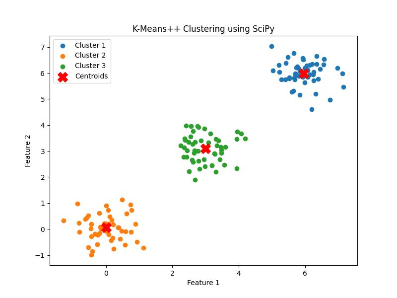
SciPy does not directly implement K-means++ in the scipy.cluster.vq module but it can be used through the kmeans function by setting the minit parameter to '++'. This ensures that the centroids are initialized using the K-means++ strategy. Below is the example −

import numpy as np
from scipy.cluster.vq import kmeans2
import matplotlib.pyplot as plt

# Generate some synthetic data
np.random.seed(0)
data = np.vstack([np.random.normal(0, 0.5, (50, 2)), 
                  np.random.normal(3, 0.5, (50, 2)), 
                  np.random.normal(6, 0.5, (50, 2))])

# Number of clusters
k = 3

# Perform K-means++ clustering
centroids, labels = kmeans2(data, k, minit='++')

# Plot the results
plt.figure(figsize=(8, 6))
for i in range(k):
    plt.scatter(data[labels == i, 0], data[labels == i, 1], label=f'Cluster {i+1}')
plt.scatter(centroids[:, 0], centroids[:, 1], c='red', marker='X', s=200, label='Centroids')
plt.title('K-Means++ Clustering using SciPy')
plt.xlabel('Feature 1')
plt.ylabel('Feature 2')
plt.legend()
plt.show()

print(f"Centroids:\n{centroids}")

Here is the output of the K-means++ clustering −

Centroids:
[[5.95346338 5.98730436]
 [0.00840308 0.05140493]
 [2.99063924 3.09137373]]

Vector quantization

Vector quantization involves partitioning a large set of vectors into a smaller set of clusters. Each vector in the dataset is approximated by the nearest representative vector which is known as a codebook vector or centroid. The set of these codebook vectors is called a codebook.

Vector quantization (VQ) is a technique in signal processing and machine learning used to compress and encode vector data by mapping it to a finite set of representative vectors. It is widely used in data compression, pattern recognition and clustering.

How Vector Quantization Works

Here are the steps which shows how the Vector quantization works −

Training
• Initialization: Choose an initial set of codebook vectors. This can be done randomly or using methods like K-means clustering.
• Assignment: Assign each data vector to the nearest codebook vector.
• Update: Recalculate the codebook vectors as the mean of all vectors assigned to each codebook vector.
• Iteration: Repeat the assignment and update steps until convergence, meaning that the codebook vectors no longer change significantly.

Encoding

After training each data vector is encoded by its index in the codebook rather than by the vector itself. This reduces the amount of data needed to represent the original data.

Decoding

To reconstruct the data we have to replace each index with the corresponding codebook vector. This results in a compressed approximation of the original data.

Example

Heres an example of vector quantization using K-means clustering from scipy.cluster.vq which effectively performs vector quantization −

import numpy as np
from scipy.cluster.vq import kmeans, vq
import matplotlib.pyplot as plt

# Generate synthetic data
np.random.seed(0)
data = np.vstack([np.random.normal(0, 0.5, (100, 2)), 
                  np.random.normal(3, 0.5, (100, 2)), 
                  np.random.normal(6, 0.5, (100, 2))])

# Number of codebook vectors (clusters)
k = 3

# Perform K-means clustering to get codebook vectors
centroids, distortion = kmeans(data, k)

# Assign each sample to a cluster
labels, _ = vq(data, centroids)

# Plot the results
plt.figure(figsize=(8, 6))
for i in range(k):
    plt.scatter(data[labels == i, 0], data[labels == i, 1], label=f'Cluster {i+1}')
plt.scatter(centroids[:, 0], centroids[:, 1], c='red', marker='X', s=200, label='Codebook Vectors')
plt.title('Vector Quantization using K-means')
plt.xlabel('Feature 1')
plt.ylabel('Feature 2')
plt.legend()
plt.show()

print(f"Codebook Vectors:\n{centroids}")
print(f"Distortion: {distortion}")

The output of the Vector quantization using K-Means Clustering is given below −

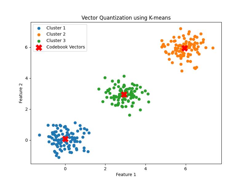
Codebook Vectors:
[[-4.78840902e-04  7.13893340e-02]
 [ 5.94382124e+00  5.94843116e+00]
 [ 2.92846083e+00  2.94352468e+00]]
Distortion: 0.6249447014860251