SciPy - Laplacian Filter

---

---

Laplacian Filter in SciPy

The Laplacian filter is a second-order derivative filter used to highlight regions of rapid intensity change in an image such as edges. It calculates the Laplacian which is the sum of the second derivatives in the x and y directions.

For a 2D image I(x,y), mathematically the Laplacian is given as follows −

This operation captures regions where the intensity changes abruptly. When we want to implement the Laplacian filter using scipy library then we can use the function scipy.ndimage.laplace().

Syntax

Following is the syntax of the scipy.ndimage.laplace() function −

scipy.ndimage.laplace(input, output=None, mode='reflect', cval=0.0)

Following are the parameters of the function scipy.ndimage.laplace() −

• input: The input array i.e., image to which the filter is applied.
• output(optional): An array to store the result. If not provided then a new array is created.
• mode: This parameter defines how the input array is extended at its boundaries. The modes can be 'reflect', 'constant', 'nearest', 'mirror' and 'wrap'.
• cval: This is a value to fill past edges if mode='constant'. Default value is 0.0.

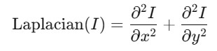
Basic Laplacian Filter on a Synthetic Image

Following is an example which shows how to apply the basic Laplacian Filter on a synthetic image using the function scipy.ndimage.laplace() −

import numpy as np
import matplotlib.pyplot as plt
from scipy import ndimage

# Create a synthetic checkerboard pattern
x = np.indices((100, 100)).sum(axis=0) % 2
image = x.astype(float)

# Apply the Laplacian filter
laplacian = ndimage.laplace(image)

# Plot
plt.figure(figsize=(10, 5))
plt.subplot(1, 2, 1)
plt.title("Checkerboard Pattern")
plt.imshow(image, cmap='gray')
plt.axis('off')

plt.subplot(1, 2, 2)
plt.title("Laplacian Filter")
plt.imshow(laplacian, cmap='gray')
plt.axis('off')
plt.show()

Following is the output of the basic laplacian filter applied on the given image −

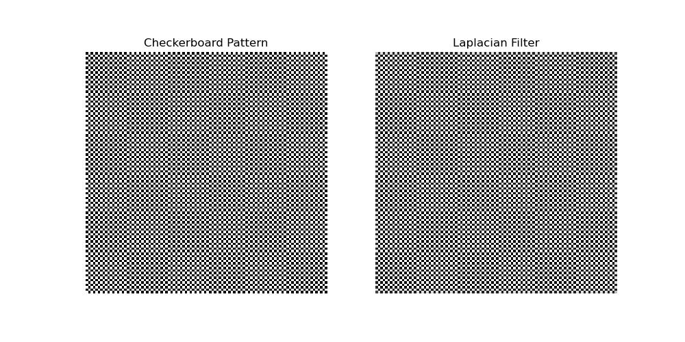
Laplacian Filter with Pre-Smoothing

The Laplacian filter with pre-smoothing is a technique in image processing where a Gaussian filter is applied to reduce noise before applying the Laplacian filter. This combination is effective for edge detection while minimizing noise artifacts. Following is the example applying a Gaussian filter before the Laplacian filter on a noisy image −

import numpy as np
from scipy import ndimage
import matplotlib.pyplot as plt

# Create a noisy image
np.random.seed(42)
image = np.random.random((100, 100))

# Apply Gaussian smoothing before Laplacian filter
smoothed = ndimage.gaussian_filter(image, sigma=2)
laplacian = ndimage.laplace(smoothed)

# Plot
plt.figure(figsize=(15, 5))
plt.subplot(1, 3, 1)
plt.title("Original Noisy Image")
plt.imshow(image, cmap='gray')
plt.axis('off')

plt.subplot(1, 3, 2)
plt.title("Smoothed Image")
plt.imshow(smoothed, cmap='gray')
plt.axis('off')

plt.subplot(1, 3, 3)
plt.title("Laplacian Filter (Post-Smoothing)")
plt.imshow(laplacian, cmap='gray')
plt.axis('off')
plt.show()

Following is the output of the applying the Laplace Filter with Pre - smoothing −

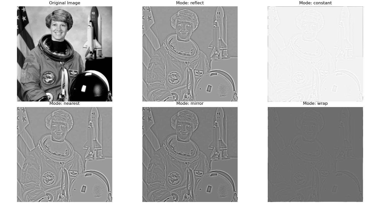
Laplacian Filter with Boundary Modes

In the Laplacian filter and Gaussian smoothing the boundary modes control how the edges of the image are handled during the convolution. This is important because the filter operates beyond the original image's boundaries. Here in this example we are passing the mode parameter to the scipy.ndimage.laplace() function −

import numpy as np
import matplotlib.pyplot as plt
from scipy import ndimage
from skimage import data, color

# Step 1: Load image
image = color.rgb2gray(data.astronaut())  # Convert to grayscale

# Step 2: Pre-smoothing with Gaussian filter
sigma = 2
smoothed_image = ndimage.gaussian_filter(image, sigma=sigma)

# Step 3: Apply Laplacian filter with different modes
modes = ['reflect', 'constant', 'nearest', 'mirror', 'wrap']
results = {}

for mode in modes:
    laplacian = ndimage.laplace(smoothed_image, mode=mode, cval=0)  # cval=0 for 'constant'
    results[mode] = laplacian

# Step 4: Visualize the results
plt.figure(figsize=(15, 10))
plt.subplot(2, 3, 1)
plt.title("Original Image")
plt.imshow(image, cmap='gray')
plt.axis('off')

for i, mode in enumerate(modes, start=2):
    plt.subplot(2, 3, i)
    plt.title(f"Mode: {mode}")
    plt.imshow(results[mode], cmap='gray')
    plt.axis('off')

plt.tight_layout()
plt.show()

Following is the output of the applying the Laplace Filter with Pre - smoothing −