SciPy - Linear Curve Fitting

---

---

Linear Curve Fitting is a fundamental statistical technique used to model the relationship between two variables by fitting a linear equation to the observed data. In the view of SciPy linear curve fitting typically involves in minimizing the differences i.e., residuals between observed data points and those predicted by a linear model.

Lets see in detail about Linear Curve Fitting mathematical foundation and the tools provided by SciPy.

Understanding Linear Curve Fitting

Understanding linear curve fitting involves grasping the fundamental concepts, methods and applications of fitting a linear model to a dataset. Here are the key aspects of linear curve fitting.

Linear Relationship

A linear relationship implies that changes in one variable result in proportional changes in another variable. Mathematically it can be expressed as follows −

y = mx+b

Where −

• y is the dependent variable i.e. what we are trying to predict or explain.
• x is the independent variable i.e., the input or predictor.
• m is the slope of the line that indicates how much y changes for a one-unit change in x.
• b is the y-intercept i.e., the value of y when x=0.

Objectives of Linear Fitting

The goal of linear curve fitting is to find the best-fitting line that minimizes the sum of the squared residuals which is given as follows −

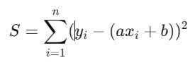
Where −

S is the sum of squared differences (residuals).

y_i are the observed values.

ax_i+b are the predicted values from the linear model.

Here are the objectives to achieve the goal of linear curve fitting −

• Understanding Relationships: Linear fitting helps to determine how changes in an independent variable (x) affect a dependent variable (y). This understanding can reveal underlying trends and patterns in empirical data which can be critical for decision-making processes.
• Prediction: Once a linear relationship is established then the model can be used to predict the value of y for any given x. This is particularly useful in fields such as economics, finance and natural sciences where forecasting based on historical data is essential.
• Modeling: Linear models provide a simple yet effective way to approximate the behavior of a system. They serve as a foundation for more complex models by allowing researchers to build on them for more nuanced analyses.
• Statistical Inference: By analyzing the slope, intercept and goodness-of-fit statistics such as ² and p-values where one can draw conclusions about the reliability and validity of the model. This helps in understanding whether the observed relationships are statistically significant or likely due to chance.
• Error Minimization: The least squares method is commonly employed to find the optimal parameters i.e., slope and intercept that minimize the residuals which is the differences between actual and predicted values. This ensures the best possible fit of the linear model to the data.
• Understanding Variability: Understanding variability helps to assess the effectiveness of the linear model. By calculating metrics such as ² analysts can determine the proportion of variance in y that is explained by x by providing insights into the model's explanatory power.
• Diagnostic Insights: Analyzing residuals and other diagnostic metrics can reveal whether the linear model is appropriate for the data or if assumptions such as linearity, homoscedasticity and normality are violated which may suggest the need for alternative modeling approaches.
.

Methods for Linear Fitting in SciPy

SciPy provides several robust methods for performing linear fitting each with its unique features, advantages and use cases. Below is a detailed overview of the methods for linear fitting in SciPy −

scipy.stats.linregress()

scipy.stats.linregress() is a function in the SciPy library used for performing simple linear regression analysis. It fits a linear model to a set of data points by providing various statistics that describe the relationship between the independent variable x and the dependent variable y. This function is particularly useful for quickly obtaining the slope, intercept, correlation coefficient, p-values and standard errors associated with the linear regression.

Syntax

Following is the syntax of using the scipy.stats.linregress() function −

scipy.stats.linregress(x, y)

Following are the parameters of the scipy.stats.linregress() function −

• x(array): The independent variable data i.e., predictor. This should be a 1D array or list of values.
• y(array): The dependent variable data i.e., response. This should also be a 1D array or list of values with the same length as x.

Example

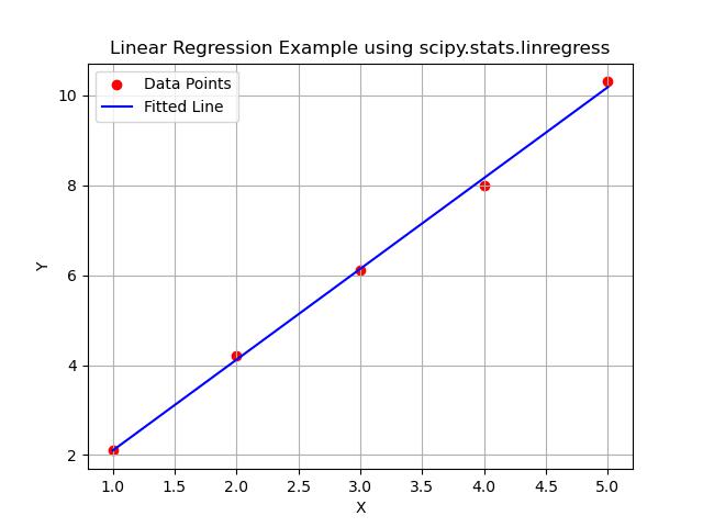
Heres a simple example showing how to use scipy.stats.linregress() function to perform linear regression and visualize the results −

import numpy as np
import matplotlib.pyplot as plt
from scipy.stats import linregress

# Sample data
x = np.array([1, 2, 3, 4, 5])
y = np.array([2.1, 4.2, 6.1, 8.0, 10.3])

# Perform linear regression
slope, intercept, r_value, p_value, std_err = linregress(x, y)

# Print the results
print(f"Slope: {slope}")
print(f"Intercept: {intercept}")
print(f"R-squared: {r_value**2}")  # R-squared value
print(f"P-value: {p_value}")
print(f"Standard Error: {std_err}")

# Create a line for plotting
x_fit = np.linspace(1, 5, 100)
y_fit = slope * x_fit + intercept

# Plot the data points and the fitted line
plt.scatter(x, y, label='Data Points', color='red')
plt.plot(x_fit, y_fit, label='Fitted Line', color='blue')
plt.xlabel('X')
plt.ylabel('Y')
plt.title('Linear Regression Example using scipy.stats.linregress')
plt.legend()
plt.grid()
plt.show()

Below is the output of the scipy.stats.linregress() function −

Slope: 2.0200000000000005
Intercept: 0.0799999999999983
R-squared: 0.9988250269264667
P-value: 1.709951883244442e-05
Standard Error: 0.039999999999992895

scipy.optimize.least_squares()

scipy.optimize.least_squares()is a function in the SciPy library that performs nonlinear least squares optimization. This function is used to minimize the sum of the squares of residuals between observed and modeled data by making it ideal for fitting models to data in various fields such as statistics, engineering and machine learning.

Syntax

Following is the syntax of using the scipy.optimize.least_squares() function −

scipy.optimize.least_squares(fun, x0, args=(), jac='2-point', bounds=(-inf, inf), method='trf', 
                              x_scale='jac', ftol=1e-8, xtol=1e-8, gtol=1e-8, max_nfev=None, 
                              verbose=0, **options)

Following are the parameters of the scipy.optimize.least_squares() function −

• fun(callable): The objective function to minimize. It should return an array of residuals f(x) where x is the vector of parameters.
• x0(array-like): Initial guess for the parameters to be optimized.
• args(tuple, optional): Extra arguments passed to the objective function fun.
• jac({'2-point, '3-point, 'cs, callable}, optional): The Jacobian matrix of the objective function. This can be provided explicitly or approximated using finite differences. The default is '2-point' which uses a two-point finite difference approximation.
• bounds(sequence, optional): Bounds on the parameters. It should be provided as a tuple of two arrays, (min, max) where each array has the same length as x0.
• method({'trf, 'dogbox, 'lm}, optional): The algorithm to use for optimization. The 'trf' and 'dogbox' methods are suitable for large problems while 'lm' is a Levenberg-Marquardt algorithm for smaller problems.
• x_scale ({jac, linear, array-like}, optional): Scaling of the variables. This can improve convergence.
• ftol, xtol, gtol (float, optional): The tolerances for termination. This algorithm will stop when these tolerances are met.
• max_nfev (int, optional): Maximum number of function evaluations.
• verbose (int, optional): Level of output. Use 1 for a summary, 2 for more detailed information.
• **options (optional): Additional options specific to the chosen method.

Example

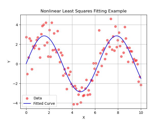
Here's an example which shows how to use scipy.optimize.least_squares() to fit a nonlinear model to data −

import numpy as np
import matplotlib.pyplot as plt
from scipy.optimize import least_squares

# Example data
x_data = np.linspace(0, 10, 100)
y_data = 3 * np.sin(x_data) + np.random.normal(size=x_data.size)

# Define the model function
def model(x, a, b):
    return a * np.sin(b * x)

# Define the residuals function
def residuals(params, x, y):
    return y - model(x, *params)

# Initial guess for parameters (a, b)
initial_params = [1.0, 1.0]

# Perform least squares fitting
result = least_squares(residuals, initial_params, args=(x_data, y_data))

# Get the optimal parameters
optimal_a, optimal_b = result.x

# Generate fitted values for plotting
y_fit = model(x_data, optimal_a, optimal_b)

# Plot the data and the fitted curve
plt.scatter(x_data, y_data, label='Data', color='red', alpha=0.5)
plt.plot(x_data, y_fit, label='Fitted Curve', color='blue')
plt.xlabel('X')
plt.ylabel('Y')
plt.title('Nonlinear Least Squares Fitting Example')
plt.legend()
plt.grid()
plt.show()

# Print the optimal parameters
print(f"Optimal parameters: a = {optimal_a}, b = {optimal_b}")

Below is the output of the scipy.optimize.least_squares() function −

Optimal parameters: a = 2.863938083609976, b = 0.9978215567742089

scipy.optimize.minimize()

The scipy.optimize.minimize() function is a versatile tool in the SciPy library used for minimizing scalar or multi-dimensional functions. It can handle a variety of optimization problems from simple unconstrained problems to complex constrained optimization tasks.

Syntax

Following is the syntax of using the scipy.optimize.minimize() function −

scipy.optimize.minimize(fun, x0, args=(), method=None, jac=None, bounds=None, constraints=(), 
                         tol=None, options=None)

Following are the parameters of the scipy.optimize.minimize() function −

• fun(callable): The objective function to minimize.
• x0(array-like): Initial guess for the parameters.
• args(tuple, optional): Additional arguments to pass to fun.
• bounds(sequence, optional): Bounds on the parameters.
• method(optional): The optimization method to use such as 'BFGS', 'L-BFGS-B', etc.
• **options (optional): Additional options specific to the chosen method.

Example

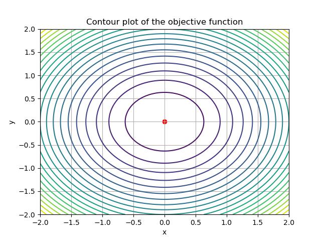
Below is a simple example of how to use scipy.optimize.minimize() to minimize a quadratic function −

import numpy as np
import matplotlib.pyplot as plt
from scipy.optimize import minimize

# Define the objective function
def objective_function(x):
    return x[0]**2 + x[1]**2  # f(x, y) = x^2 + y^2

# Initial guess
x0 = np.array([1, 1])

# Perform minimization
result = minimize(objective_function, x0)

# Print the results
print("Optimal value:", result.x)
print("Objective function value at optimal:", result.fun)

# Visualize the optimization process
x1 = np.linspace(-2, 2, 100)
x2 = np.linspace(-2, 2, 100)
X1, X2 = np.meshgrid(x1, x2)
Z = objective_function([X1, X2])

plt.contour(X1, X2, Z, levels=20)
plt.scatter(result.x[0], result.x[1], color='red')  # Optimal point
plt.title('Contour plot of the objective function')
plt.xlabel('x')
plt.ylabel('y')
plt.grid()
plt.show()

Below is the output of the scipy.optimize.minimize() function which is used to minimize the linear curve −

Optimal value: [-1.07505143e-08 -1.07505143e-08]
Objective function value at optimal: 2.311471135620994e-16