SciPy - Low Pass Filters

---

---

SciPy - Low Pass Filters

Low-pass filters are also called as Smoothing filters which are used in image processing to smooth or blur an image by reducing high-frequency components such as noise or rapid intensity changes. These filters preserve low-frequency information i.e., smooth variations while attenuating high-frequency details like edges or noise.

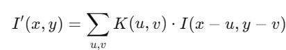
Mathematically we can give a low-pass filter which modifies the image I(x,y) by convolving it with a kernel K as follows −

Following are the different types of Low pass filters available in scipy −

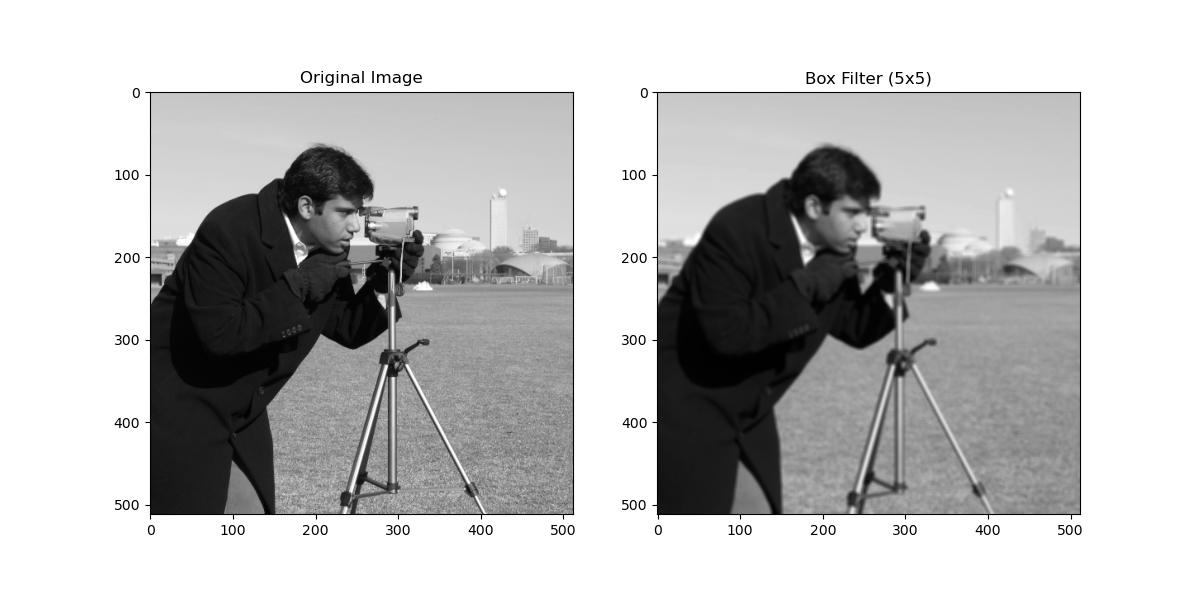
Box Filter in SciPy

A Box filter is also called as Uniform filter which computes the average intensity of all pixels in a neighborhood defined by a kernel size. It is simple and fast but may blur edges. In scipy we have the function scipy.ndimage.uniform_filter() to apply the box filter to an image. The size parameter defines the neighborhood size and large sizes result in more blur but reduce image details.

Following is an example which applies the uniform filter on an image with the help of the function scipy.ndimage.uniform_filter() −

from scipy.ndimage import uniform_filter
import matplotlib.pyplot as plt
from skimage import data

# Load an example image
image = data.camera()

# Apply a box filter (uniform filter) with a size of 5x5
filtered_image = uniform_filter(image, size=5)

# Display original and filtered images
plt.figure(figsize=(12, 6))
plt.subplot(1, 2, 1)
plt.title("Original Image")
plt.imshow(image, cmap="gray")

plt.subplot(1, 2, 2)
plt.title("Box Filter (5x5)")
plt.imshow(filtered_image, cmap="gray")
plt.show()

Below is the output of the box filter −

Gaussian Filter in SciPy

The Gaussian filter is one of the most popular low-pass filters. It uses a Gaussian kernel where pixels closer to the center of the kernel have higher weights. We have the function scipy.ndimage.guassian_filter() to use the Gaussian filter on an image.

The Gaussian kernel is defined as follows −

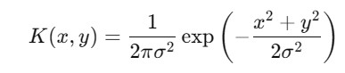
Where, is the Standard deviation of the Gaussian which controls the amount of smoothing.

is used to control the degree of smoothing where larger values result in greater blur and Gaussian smoothing is ideal for removing noise without severely blurring edges.

Below is an example which shows how to use the gaussian filter on an image with the help of the function scipy.ndimage.guassian_filter() −

from scipy.ndimage import gaussian_filter
import matplotlib.pyplot as plt
from skimage import data

# Load an example image
image = data.camera()

# Apply Gaussian filter with standard deviation sigma=2
gaussian_blurred = gaussian_filter(image, sigma=2)

# Display original and blurred images
plt.figure(figsize=(12, 6))
plt.subplot(1, 2, 1)
plt.title("Original Image")
plt.imshow(image, cmap="gray")

plt.subplot(1, 2, 2)
plt.title("Gaussian Filter (sigma=2)")
plt.imshow(gaussian_blurred, cmap="gray")
plt.show()

Here is the output of the Gaussian filter −

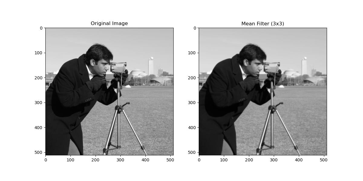
Mean Filter in SciPy

The mean filter replaces each pixel with the average of its neighbors. While effective for noise reduction it does not preserve edges well.

The kernel averages the pixel intensities which lead to a simple smoothing effect and larger kernels increase the smoothing effect but at the cost of edge detail.

In this example we are applying the mean filter to the given input image by using the function scipy.ndimage.convolve() −

from scipy.ndimage import convolve
import numpy as np
import matplotlib.pyplot as plt
from skimage import data

# Load an example image
image = data.camera()

# Define a mean filter kernel (3x3)
mean_kernel = np.ones((3, 3)) / 9

# Apply mean filter using convolution
mean_filtered = convolve(image, mean_kernel)

# Display original and mean-filtered images
plt.figure(figsize=(12, 6))
plt.subplot(1, 2, 1)
plt.title("Original Image")
plt.imshow(image, cmap="gray")

plt.subplot(1, 2, 2)
plt.title("Mean Filter (3x3)")
plt.imshow(mean_filtered, cmap="gray")
plt.show()

Following is the output of the Mean filter −

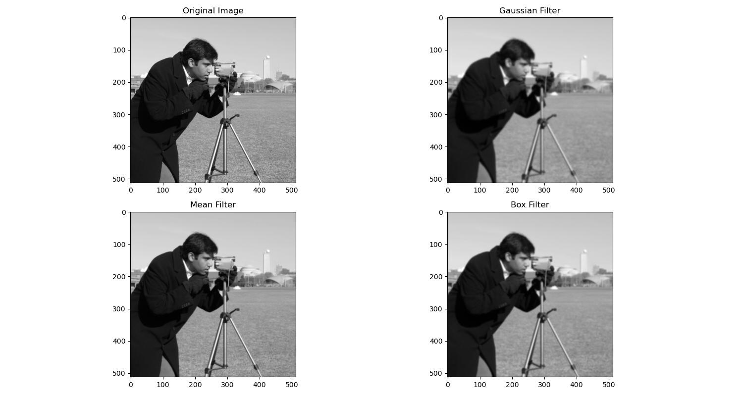
Here is an example which compares all the three different types of Low pass filters that we can use on the given input image −

from scipy import ndimage
import numpy as np
import matplotlib.pyplot as plt
from skimage import data

# Load an example image
image = data.camera()

# Define a mean filter kernel (3x3)
mean_kernel = np.ones((3, 3)) / 9

# Apply different filters and compare
gaussian = ndimage.gaussian_filter(image, sigma=2)
mean = ndimage.convolve(image, mean_kernel)
box = ndimage.uniform_filter(image, size=5)

# Display results
plt.figure(figsize=(15, 8))
plt.subplot(2, 2, 1)
plt.title("Original Image")
plt.imshow(image, cmap="gray")

plt.subplot(2, 2, 2)
plt.title("Gaussian Filter")
plt.imshow(gaussian, cmap="gray")

plt.subplot(2, 2, 3)
plt.title("Mean Filter")
plt.imshow(mean, cmap="gray")

plt.subplot(2, 2, 4)
plt.title("Box Filter")
plt.imshow(box, cmap="gray")

plt.tight_layout()
plt.show()

Following is the output of the above code for comparing the different low pass filters −