SciPy - Non Linear Curve Fitting

---

---

SciPy's non-linear curve fitting is a powerful tool in Python for estimating the parameters of a non-linear model to best fit a given set of data. This method is commonly used to model data when the relationship between the independent variable x and the dependent variable y is not a straight line.

Non-Linear Curve Fitting in SciPy

SciPy's optimize.curve_fit function from the scipy.optimize module is the main tool for non-linear curve fitting. Heres how it works −

Defining the Model Function

In non-linear curve fitting with SciPy the model function is a mathematical expression that represents the relationship between the independent variable(s) and the dependent variable(s) in our data. Its the function that we aim to fit to our data by adjusting its parameters to best match the observed values.

The model function should be defined explicitly in Python as a standard function. When using SciPys curve_fit() function this model function is passed as an argument by allowing curve_fit() function to optimize the function's parameters to fit the data.

Characteristics of the Model Function

Following are the characteristics of the Model Function −

• Non-linear form: The function is often non-linear with respect to its parameters. The most common non-linear models include exponential functions, power laws, logistic functions and other complex mathematical relationships.
• Parameters: This function must include parameters that curve_fit() function will optimize. These parameters are the variables that determine the shape of the function such as amplitude, decay rate, etc.
• Input and Output: This function must take at least two arguments namely, the independent variables which are typically given as arrays and the parameters to be optimized which are given as separate arguments.

Using the Model Function in curve_fit

To perform non-linear curve fitting with curve_fit() function in which we can pass this model function as an argument along with our data as follows −

from scipy.optimize import curve_fit
import numpy as np

def model_func(x, a, b, c):
    return a * np.exp(-b * x) + c

# Sample data
x_data = np.linspace(0, 4, 50)
y_data = model_func(x_data, 2.5, 1.3, 0.5) + 0.2 * np.random.normal(size=len(x_data))

# Fit the curve
initial_guesses = [1.0, 1.0, 1.0]
popt, pcov = curve_fit(model_func, x_data, y_data, p0=initial_guesses)
print(popt)
print(pcov)

Following is the output of the above code −

[2.373493   1.3085931  0.55674186]
[[ 0.00991781  0.00433252 -0.00052527]
 [ 0.00433252  0.01414914  0.00379678]
 [-0.00052527  0.00379678  0.00191205]]

Provide Initial Parameter Estimates

In non-linear curve fitting the initial parameter estimates or initial guesses are starting values for the model parameters that help the optimization algorithm converge to the best fit. Since non-linear fitting involves iterative optimization by having reasonable initial guesses can significantly affect the speed and success of the fitting process.

Why Initial Estimates Are Important?

Here are the reasons why initial estimates are important −

• Convergence: Non-linear optimization methods like the one used by curve_fit() function may not converge to the correct solution without good starting points.
• Efficiency: Good estimates can reduce the number of iterations required by making the fitting faster.
• Avoiding Local Minima: Some models can have multiple solutions so an appropriate initial guess can help the algorithm avoid "getting stuck" in a local minimum instead of finding the global best fit.

How to Choose Initial Parameter Estimates?

Choosing initial values can vary depending on the model and data but here are some general approaches −

• Estimate from Data: Use prior knowledge or approximate values based on our data. For instance let's consider −
• If fitting an exponential decay curve y = a.e^-bx+c the initial value y at x = 0 could guide the choice for a.
• For linear or polynomial models then use the first few data points to estimate the slope or intercept.
• Try Common Starting Values: For some parameters typical values like 1.0, 0.0 or other neutral values can be a reasonable start if there is no strong prior information.
• Trial and Error: If a fit doesnt converge or gives a poor result, experiment with different starting values until we find a set that works well.

Implementing Initial Estimates with curve_fit()

Here is the example of implementing initial estimates with the curve_fit() function −

import numpy as np
from scipy.optimize import curve_fit

# Define the model function
def model_func(x, a, b, c):
    return a * np.exp(-b * x) + c

# Generate sample data
x_data = np.linspace(0, 4, 50)
y_data = model_func(x_data, 2.5, 1.3, 0.5) + 0.2 * np.random.normal(size=len(x_data))

# Initial guesses for parameters: a, b, c
initial_guesses = [2.0, 1.0, 0.5]  # Reasonable starting values based on the data

# Fit the model to the data
popt, pcov = curve_fit(model_func, x_data, y_data, p0=initial_guesses)

# Output the optimized parameters
print("Optimized parameters:", popt)

Here is the output of implementing initial estimates with curve_fit() function −

Optimized parameters: [2.44641902 1.25183589 0.51762444]

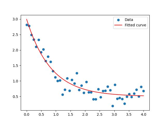
Fit the Curve

Using curve_fit() function we can fit the curve. This function tries to find the best parameters that minimize the difference between the model predictions and the actual data.

Here is the example of using curve_fit() function to fit an exponential decay function −

import numpy as np
from scipy.optimize import curve_fit
import matplotlib.pyplot as plt

# Define a non-linear function (exponential decay)
def model_func(x, a, b, c):
    return a * np.exp(-b * x) + c

# Generate synthetic data (for illustration)
x_data = np.linspace(0, 4, 50)
y_data = model_func(x_data, 2.5, 1.3, 0.5) + 0.2 * np.random.normal(size=len(x_data))

# Fit the data to the model
initial_guesses = [1.0, 1.0, 1.0]  # Initial parameter guesses for a, b, c
popt, pcov = curve_fit(model_func, x_data, y_data, p0=initial_guesses)

# Extract the fitted parameters
a_fitted, b_fitted, c_fitted = popt

# Plot the data and the fitted curve
plt.scatter(x_data, y_data, label='Data')
plt.plot(x_data, model_func(x_data, *popt), color='red', label='Fitted curve')
plt.legend()
plt.show()

Here is the output of fitting the non linear curve with the help of curve_fit() function −

Obtain Fitted Parameters

The curve_fit() function returns the optimal parameters along with a covariance matrix that provides information about the fit's accuracy.

Here is the example of getting the fitted parameters of the non linear curve with the help of curve_fit() function −

import numpy as np
from scipy.optimize import curve_fit
import matplotlib.pyplot as plt

# Define the model function
def model_func(x, a, b, c):
    return a * np.exp(-b * x) + c

# Generate synthetic data
x_data = np.linspace(0, 4, 50)
y_data = model_func(x_data, 2.5, 1.3, 0.5) + 0.2 * np.random.normal(size=len(x_data))

# Fit the model to the data
initial_guesses = [1.0, 1.0, 1.0]
popt, pcov = curve_fit(model_func, x_data, y_data, p0=initial_guesses)

# Retrieve the fitted parameters
a_fitted, b_fitted, c_fitted = popt

# Display the fitted parameters
print(f"Fitted parameters:\na = {a_fitted}\nb = {b_fitted}\nc = {c_fitted}")

Here are the output of the fitted parameters obtained with the help of curve_fit() function −

Fitted parameters:
a = 2.5673199143371517
b = 1.3548808337833609
c = 0.5102248520438042