SciPy - Oscillatory Functions

---

---

What are Oscillatory Functions?

Oscillatory functions are functions that exhibit repeated fluctuations between certain values which often in a periodic manner. These functions are common in fields such as signal processing, physics and engineering.

In SciPy, oscillatory functions are such as sine, cosine and other trigonometric functions can be handled effectively using various tools for numerical integration, optimization and signal processing.

In numerical computation the oscillatory functions can present challenges especially when dealing with integration over large intervals, as the frequent sign changes can lead to cancellation errors or difficulties in convergence.

SciPy provides specialized methods to handle such functions efficiently particularly in the context of integration and solving differential equations. Some common examples of oscillatory functions are sine and cosine functions, Bessel functions and other periodic signals.

Characteristics of Oscillatory Functions

The below characteristics of Oscillatory Functions are essential in various fields such as signal processing, physics and electrical engineering where oscillatory functions model waves, vibrations and alternating currents −

• Periodicity: Oscillatory functions often repeat their values at regular intervals which is called as the period. For example when functions like sine and cosine exhibit periodic behavior with a fixed interval of 2.
• Alternating Signs: The Oscillatory functions fluctuate between positive and negative values. As they oscillate, they alternate between peaks i.e., maximum values and troughs i.e., minimum values.
• Amplitude: This refers to the maximum absolute value the function can reach. Oscillatory functions have peaks and troughs determined by this amplitude.
• Frequency: This defines how many oscillations or cycles occur within a unit interval. Higher frequency indicates more oscillations over the same interval.
• Damping (Optional): Some oscillatory functions like damped oscillations exhibit a decrease in amplitude over time due to damping factors which can be modeled with exponential terms.
• Symmetry: Many oscillatory functions exhibit symmetry such as even i.e., symmetric around the y-axis or odd i.e., symmetric around the origin behavior especially trigonometric functions such as sine and cosine.
• Phase Shift: The phase shift of an oscillatory function refers to a horizontal displacement in the function's graph by shifting the position of its peaks and troughs.

Handling Oscillatory Functions in SciPy

Oscillatory functions are common in various scientific computations particularly in physics and engineering. Due to their repetitive nature which accurately integrating or analyzing these functions can be challenging. SciPy offers tools and strategies to handle oscillatory behavior efficiently.

By adapting the integration approach or applying appropriate methods the SciPy effectively manages the challenges posed by oscillatory functions. Here the key approaches in detail −

• Quad Function for Integration: SciPys quad function can handle oscillatory integrals. While quad automatically adapts to oscillations it can sometimes struggle with highly oscillatory functions so extra care or specific methods might be necessary. Here is the example of handling the oscillatory function using quad function −

  import numpy as np
  from scipy.integrate import quad
  
  # Define an oscillatory function
  def oscillatory_func(x):
      return np.sin(100 * x)
  
  # Perform integration
  result, error = quad(oscillatory_func, 0, np.pi)
  print("Integral result:", result)
  

  Here is the output of the quad function for integration −

  Integral result: 2.3480880169895062e-15
  

• Oscillatory Weight Functions: The quad() function allows specifying a weight for integration which can help in handling oscillatory functions more efficiently by compensating for rapid changes.
• Avoiding Precision Loss: For functions with very high frequencies the precision loss can occur due to the rapid oscillations. In such cases breaking the integration range into smaller sub-ranges may yield to better accuracy.
• Specialized Methods: In some cases of Highly Oscillatory Functions the methods such as Levin integration or other specialized algorithms are recommended. Though SciPy doesn't directly offer these but other packages or custom implementations may be used for high frequency oscillatory functions.

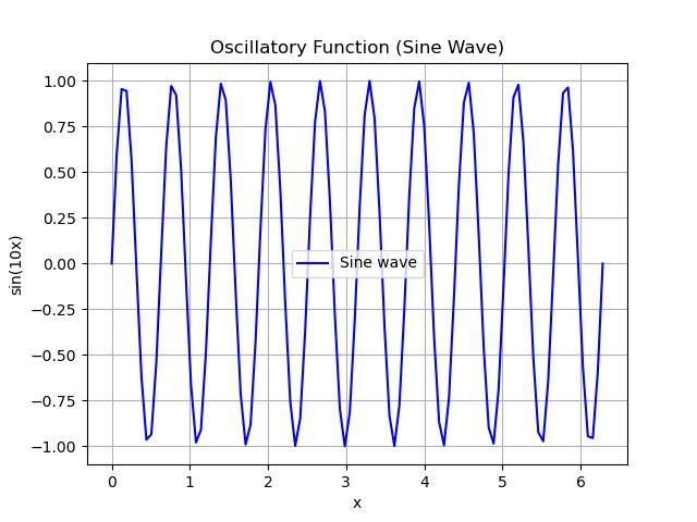
Simple Oscillatory function

In this example we define a simple sine wave function which is a classic example of an oscillatory function. We'll plot the sine wave using Matplotlib and then integrate it over a specific interval using SciPy −

import numpy as np
import matplotlib.pyplot as plt
from scipy.integrate import quad

# Define the oscillatory function (sine wave)
def oscillatory_func(x):
    return np.sin(10 * x)  # A sine wave with frequency 10

# Generate x values for plotting
x_values = np.linspace(0, 2 * np.pi, 100)
y_values = oscillatory_func(x_values)

# Plotting the oscillatory function
plt.plot(x_values, y_values, label="Sine wave", color='blue')
plt.title('Oscillatory Function (Sine Wave)')
plt.xlabel('x')
plt.ylabel('sin(10x)')
plt.grid(True)
plt.legend()
plt.show()

# Perform integration over the interval [0, 2p]
result, error = quad(oscillatory_func, 0, 2 * np.pi)
print("Integral of sin(10x) over [0, 2p]:", result)

Here is the output of the simple oscillatory function using scipy −

Types of Oscillatory Functions in SciPy

Here are the different types of Oscillatory functions available in Scipy −

Function Name	Description
Sine Wave	A basic periodic oscillatory function that repeats at regular intervals.
Cosine Wave	Similar to sine wave but shifted by a phase of /2.
Fourier Series	A series of sine and cosine functions representing complex periodic signals.
Bessel Function	A type of oscillatory function that occurs in many physical problems such as waves.
Airy Function	Oscillates but decays for large values of the input, used in quantum mechanics.
Modified Bessel Function	Oscillates but grows exponentially for large values of the input.

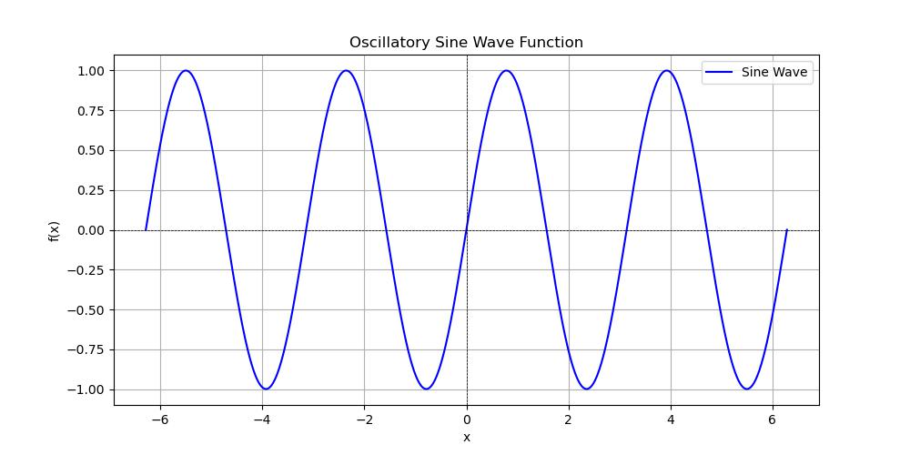
Sine Wave Oscillatory Function

In SciPy an oscillatory sine wave function refers to a periodic function that fluctuates between a maximum and a minimum value over a specified interval. The sine function represented mathematically as follows −

f(x) = A . sin(Bx + C) + D

Where, A is the amplitude which determines the peak height of the wave, B affects the frequency of oscillation i.e., number of cycles in a unit interval, C is the phase shift which determines where the wave starts along the x-axis and D is the vertical shift which moves the entire function up or down.

Here's a simple example of how to generate and plot an oscillatory sine wave function using SciPy and Matplotlib −

import numpy as np
import matplotlib.pyplot as plt
from scipy import integrate

# Define the sine wave function
def sine_wave(x, A=1, B=1, C=0, D=0):
    return A * np.sin(B * x + C) + D

# Set parameters
A = 1   # Amplitude
B = 2   # Frequency
C = 0   # Phase shift
D = 0   # Vertical shift

# Define the limits of integration
lower_limit = 0
upper_limit = 2 * np.pi

# Use scipy.integrate.quad to integrate the sine wave over one period
integral, error = integrate.quad(sine_wave, lower_limit, upper_limit, args=(A, B, C, D))

# Output the result of the integration
print(f"Integral of sine wave from {lower_limit} to {upper_limit} is: {integral:.5f}")
print(f"Estimated error: {error:.5f}")

# Generate points for plotting
x = np.linspace(0, 2 * np.pi, 1000)
y = sine_wave(x, A, B, C, D)

# Plot the sine wave
plt.plot(x, y, label=f'Sine Wave (A={A}, B={B})', color='blue')
plt.title('Oscillatory Sine Wave Function')
plt.xlabel('x')
plt.ylabel('f(x)')
plt.axhline(0, color='black', lw=0.5, ls='--')
plt.axvline(0, color='black', lw=0.5, ls='--')
plt.grid(True)
plt.legend()
plt.show()

Following is the output of the Oscillatory Sine function using scipy −

Integral of sine wave from 0 to 6.283185307179586 is: -0.00000
Estimated error: 0.00000

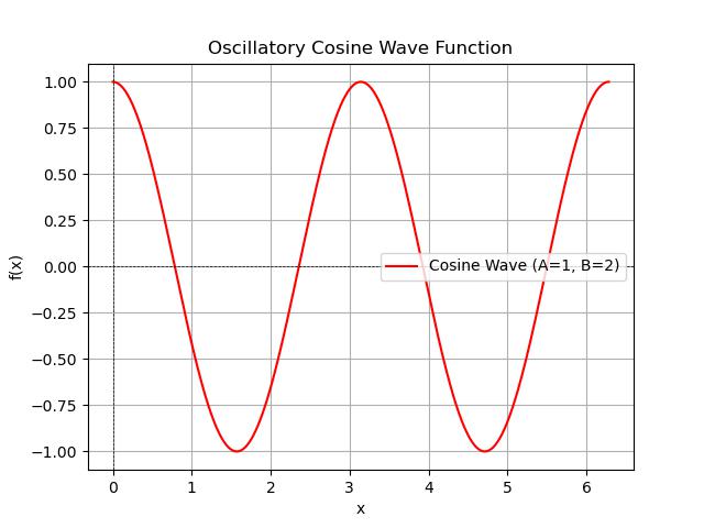
Cosine Wave Oscillatory Function

An Oscillatory cosine function in SciPy refers to a function that exhibits oscillatory behavior which is characterized by regular and repeated fluctuations in its values. Specifically the cosine function is a periodic function defined mathematically as follows −

f(x) = A . cos(Bx + C) + D

Where, A is the amplitude which determines the peak height of the wave, B affects the frequency of oscillation i.e., number of cycles in a unit interval, C is the phase shift which determines how much the function is shifted horizontally and D is the vertical shift which determines how much the function shifted vertically.

Key Features of Oscillatory Cosine Wave

Below are the key features of the Oscillatory Cosine Wave in scipy −

• Periodic Nature: The cosine function repeats its values at regular intervals, with a period given by 2/.
• Amplitude: The amplitude determines how high and low the function oscillates. A larger amplitude results in greater peaks and troughs.
• Frequency: The frequency indicates how quickly the function oscillates. A higher frequency results in more cycles in a given interval.
• Applications: Oscillatory functions such as cosine functions are commonly used in various fields such as signal processing, physics and engineering to model waveforms, vibrations and periodic phenomena.

Following is the simple example of how to generate and plot an oscillatory cosine wave function using SciPy −

import numpy as np
import matplotlib.pyplot as plt
from scipy import integrate

# Define the cosine wave function
def cosine_wave(x, A=1, B=1, C=0, D=0):
    return A * np.cos(B * x + C) + D

# Set parameters
A = 1   # Amplitude
B = 2   # Frequency
C = 0   # Phase shift
D = 0   # Vertical shift

# Define the limits of integration
lower_limit = 0
upper_limit = 2 * np.pi

# Use scipy.integrate.quad to integrate the cosine wave over one period
integral, error = integrate.quad(cosine_wave, lower_limit, upper_limit, args=(A, B, C, D))

# Output the result of the integration
print(f"Integral of cosine wave from {lower_limit} to {upper_limit} is: {integral:.5f}")
print(f"Estimated error: {error:.5f}")

# Generate points for plotting
x = np.linspace(0, 2 * np.pi, 1000)
y = cosine_wave(x, A, B, C, D)

# Plot the cosine wave
plt.plot(x, y, label=f'Cosine Wave (A={A}, B={B})', color='red')
plt.title('Oscillatory Cosine Wave Function')
plt.xlabel('x')
plt.ylabel('f(x)')
plt.axhline(0, color='black', lw=0.5, ls='--')
plt.axvline(0, color='black', lw=0.5, ls='--')
plt.grid(True)
plt.legend()
plt.show()

Following is the output of the Oscillatory Sine function using scipy −

Integral of cosine wave from 0 to 6.283185307179586 is: -0.00000
Estimated error: 0.00000

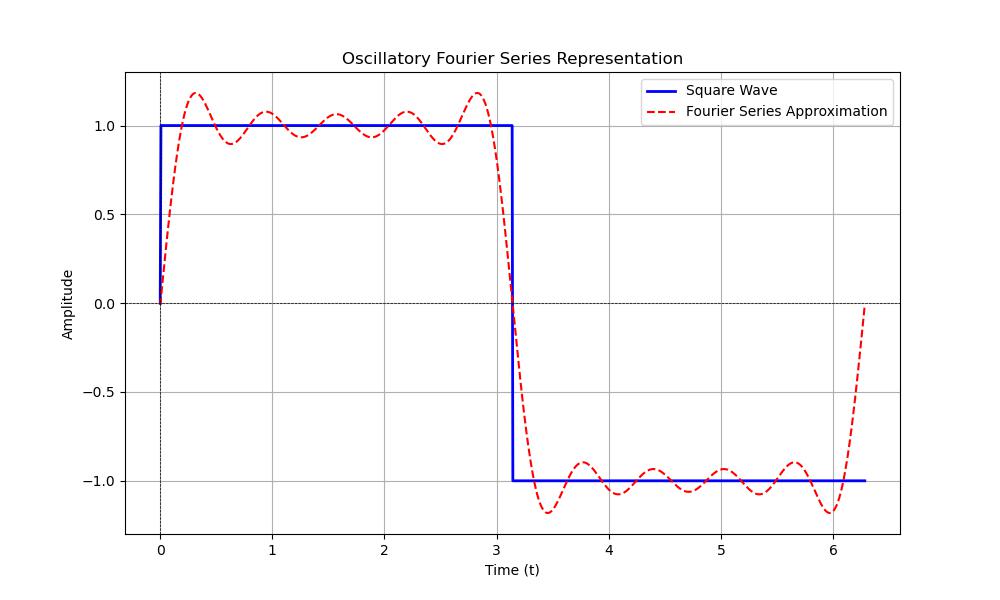
Fourier series Oscillatory Function

The Fourier series is a way to represent a periodic function as a sum of sine and cosine functions. In SciPy we can analyze oscillatory functions using Fourier series by leveraging the Fast Fourier Transform (FFT).

Here's an example showing how to create a Fourier series for an oscillatory function using SciPy −

import numpy as np
import matplotlib.pyplot as plt

# Define the time variable and the oscillatory function
t = np.linspace(0, 2 * np.pi, 1000)  # Time variable
A = 1  # Amplitude
frequency = 1  # Frequency of the oscillatory function

# Create a composite function (e.g., a square wave)
square_wave = A * np.sign(np.sin(frequency * t))

# Compute the Fourier series coefficients
n_terms = 10  # Number of terms in the Fourier series
fourier_coefficients = np.zeros((n_terms, 2))

for n in range(1, n_terms + 1):
    # Calculate coefficients for sine and cosine terms
    a_n = (1 / np.pi) * np.trapz(square_wave * np.cos(n * t), t)  # Cosine coefficients
    b_n = (1 / np.pi) * np.trapz(square_wave * np.sin(n * t), t)  # Sine coefficients
    fourier_coefficients[n - 1] = [a_n, b_n]

# Reconstruct the function using the Fourier series
fourier_series = np.zeros_like(t)

for n in range(1, n_terms + 1):
    a_n, b_n = fourier_coefficients[n - 1]
    fourier_series += a_n * np.cos(n * t) + b_n * np.sin(n * t)

# Plot the original function and its Fourier series approximation
plt.figure(figsize=(10, 6))
plt.plot(t, square_wave, label='Square Wave', color='blue', linewidth=2)
plt.plot(t, fourier_series, label='Fourier Series Approximation', color='red', linestyle='--')
plt.title('Oscillatory Fourier Series Representation')
plt.xlabel('Time (t)')
plt.ylabel('Amplitude')
plt.axhline(0, color='black', lw=0.5, ls='--')
plt.axvline(0, color='black', lw=0.5, ls='--')
plt.grid(True)
plt.legend()
plt.show()

Here is the output of the Oscillatory FFT series function using scipy −

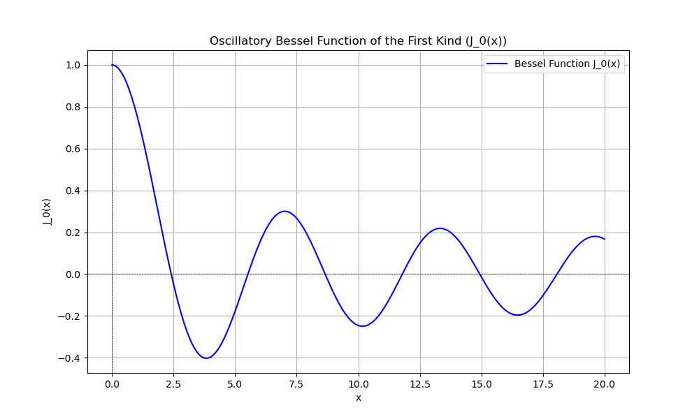
Bessel Function

The Bessel functions are a family of solutions to Bessel's differential equation and are commonly encountered in problems with cylindrical or spherical symmetry. In SciPy we can compute Bessel functions using the scipy.special module.

These functions are oscillatory in nature and they have applications in wave propagation, static potentials and signal processing among other fields.

This example shows how to compute and plot a Bessel function of the first kind _n(x) which is one of the most common types of Bessel functions −

import numpy as np
import matplotlib.pyplot as plt
from scipy.special import jn  # Bessel function of the first kind

# Define the order of the Bessel function (n) and the x-values
n = 0  # Order of the Bessel function
x = np.linspace(0, 20, 1000)  # Range of x-values

# Compute the Bessel function of the first kind
bessel_function = jn(n, x)

# Plotting the Bessel function
plt.figure(figsize=(10, 6))
plt.plot(x, bessel_function, label=f'Bessel Function J_{n}(x)', color='blue')
plt.title(f'Oscillatory Bessel Function of the First Kind (J_{n}(x))')
plt.xlabel('x')
plt.ylabel(f'J_{n}(x)')
plt.axhline(0, color='black', lw=0.5, ls='--')
plt.axvline(0, color='black', lw=0.5, ls='--')
plt.grid(True)
plt.legend()
plt.show()

Here is the output of the Oscillatory Bessel Function using scipy −

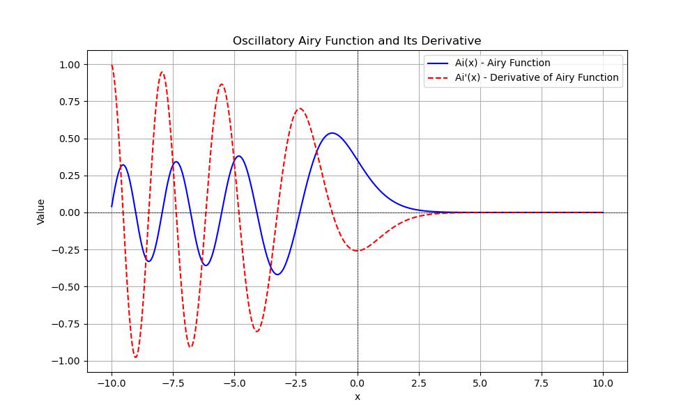
Airy Function

The Airy function is a special function used to solve differential equations and is characterized by oscillatory behavior for negative values of its argument. In SciPy we can compute the Airy function using the scipy.special.airy() function.

It returns the values of the Airy function along with its derivative and other related functions.

Characteristics of the Airy Function

Here are the characteristics of the Airy Funtcion in scipy −

• Oscillatory Behavior: For negative values of x, the Airy function behaves like a damped oscillatory wave.
• Decay: For negative values of x, the Airy function behaves like a damped oscillatory wave.
• Oscillatory Behavior: For positive values of x, the Airy function decays rapidly.
• Applications: Airy functions are commonly used in quantum mechanics, optics and signal processing especially when solving differential equations with turning points.

Here is the example of working with the Oscillatory Airy Function in scipy −

import numpy as np
import matplotlib.pyplot as plt
from scipy.special import airy

# Define the range of x values
x = np.linspace(-10, 10, 1000)

# Calculate the Airy function Ai(x) and its derivative
Ai, Aip, Bi, Bip = airy(x)

# Plotting the Airy Ai function (oscillatory for negative x)
plt.figure(figsize=(10, 6))
plt.plot(x, Ai, label='Ai(x) - Airy Function', color='blue')
plt.plot(x, Aip, label="Ai'(x) - Derivative of Airy Function", color='red', linestyle='--')

# Title and labels
plt.title('Oscillatory Airy Function and Its Derivative')
plt.xlabel('x')
plt.ylabel('Value')
plt.axhline(0, color='black', lw=0.5, ls='--')
plt.axvline(0, color='black', lw=0.5, ls='--')
plt.grid(True)
plt.legend()

# Show the plot
plt.show()

Here is the output of the Oscillatory Bessel Function using SciPy −

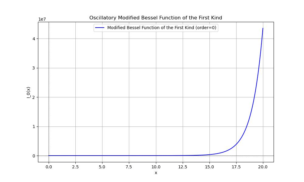
Modified Bessel Function

The Modified Bessel Function is the First Kind which is often used in various fields including physics and engineering especially when dealing with oscillatory problems in cylindrical coordinates. In SciPy we can use the scipy.special module to compute these functions.

Following is the example of working with the Oscillatory Modified Bessel Function in SciPy −

import numpy as np
import matplotlib.pyplot as plt
from scipy.special import iv  # Import the Modified Bessel function of the first kind

# Define the range for the x values
x = np.linspace(0, 20, 1000)

# Define the order of the Bessel function
order = 0  # You can change this to 1, 2, etc., for higher orders

# Compute the Modified Bessel function of the first kind
bessel_values = iv(order, x)

# Plot the results
plt.figure(figsize=(10, 6))
plt.plot(x, bessel_values, label=f'Modified Bessel Function of the First Kind (order={order})', color='blue')
plt.title('Oscillatory Modified Bessel Function of the First Kind')
plt.xlabel('x')
plt.ylabel(f'I_{order}(x)')
plt.axhline(0, color='black', lw=0.5, ls='--')
plt.axvline(0, color='black', lw=0.5, ls='--')
plt.grid(True)
plt.legend()
plt.show()

Here is the output of the Oscillatory Bessel Function using scipy −