SciPy Partial Differential Equations (PDEs)

---

---

Partial Differential Equations (PDEs) in SciPy refer to the use of numerical methods to solve equations involving partial derivatives of functions with more than one variable. PDEs describe a wide range of phenomena in physics, engineering and other fields such as heat conduction, wave propagation and fluid dynamics.

SciPy doesn't have built-in solvers for PDEs but it supports numerical methods such as finite difference and finite element methods with the use of external libraries for approximating solutions. PDEs can also be transformed into systems of ordinary differential equations (ODEs) which can be solved using SciPys ODE solvers like solve_ivp0.

For more complex PDEs the users often rely on external libraries such as FiPy, Fenics or custom implementations for advanced numerical solutions. However SciPy can be used as a foundation for solving simpler PDE problems by discretizing the domain and applying numerical techniques to approximate solutions.

Methods of Solving PDEs in scipy

We already discussed that sciPy itself doesnt have a dedicated PDE solver but it offers support for boundary value problems, ordinary differential equations and finite difference schemes that can be used for solving PDEs. Here are the key methods and approaches commonly used in combination with SciPy for PDEs −

Finite Difference Method(FDM)

The Finite Difference Method (FDM) is a numerical technique used to approximate solutions to Partial Differential Equations (PDEs) by replacing derivatives with finite differences.

It works by discretizing the continuous domain (time, space) into a grid and approximating the derivatives of the function at each point on the grid using neighboring points. This converts the PDE into a system of algebraic equations which can be solved numerically.

Steps of FDM

Following are the steps of FDM for implementing it in Scipy −

• Discretization of the Domain: The continuous domain i.e., time or space is divided into a grid of discrete points. For example a spatial domain can be divided into N equally spaced intervals.
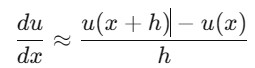
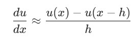
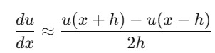
• Approximating Derivatives: Derivatives in the PDE are replaced by finite differences. Common approximations are as follows −

  Forward Difference: Approximates the derivative using the next point.

  

  Backward Difference: Uses the previous point.

  

  Central Difference: Uses the average of the next and previous points for better accuracy.

  
• Set Up the Discretized Equations: After substituting the finite difference approximations into the PDE a system of algebraic equations is obtained, with each equation corresponding to a point on the grid.
• Solve the Algebraic System: The resulting system of equations is solved using numerical methods like matrix solvers, iterative methods to approximate the solution of the original PDE.

Solving the Heat Equation with FDM

The heat equation describes the heat distribution over a rod. We can approximate it using FDM with help of scipy library. Let's consider the 1D heat equation as follows −

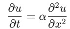
where (,) represents the temperature at position and time and is the thermal diffusivity constant.

Here's an implementation using the SciPy library to simulate the heat distribution along a rod over time −

import numpy as np
import matplotlib.pyplot as plt
from scipy.sparse import diags
from scipy.sparse.linalg import spsolve

# Parameters for the heat equation
alpha = 0.01  # Thermal diffusivity
L = 1.0       # Length of the rod
nx = 100      # Number of spatial grid points
dx = L / (nx - 1)  # Spatial step size
nt = 200      # Number of time steps
dt = 0.0005   # Time step size
time_steps = 50  # Steps to visualize
x = np.linspace(0, L, nx)  # Spatial grid

# Initial condition: Gaussian temperature distribution
u_initial = np.exp(-100 * (x - 0.5)**2)

# Create the finite difference matrix for the second spatial derivative
diagonals = [[-2] * nx, [1] * (nx - 1), [1] * (nx - 1)]
A = diags(diagonals, [0, -1, 1], shape=(nx, nx)).toarray()

# Boundary conditions: Set the edges to zero (fixed temperature)
A[0, 0] = A[-1, -1] = 1
A[0, 1] = A[-1, -2] = 0

# Time-stepping loop using FDM with an implicit scheme (backward Euler)
u = u_initial.copy()

for t in range(nt):
    # Right-hand side of the equation
    b = u + alpha * dt / dx**2 * np.dot(A, u)
    
    # Solve the linear system
    u = spsolve(A, b)
    
    # Plot every few steps
    if t % time_steps == 0:
        plt.plot(x, u, label=f't = {t * dt:.3f}')

# Final plot and visualization
plt.xlabel('x')
plt.ylabel('Temperature')
plt.title('1D Heat Equation using FDM (SciPy)')
plt.legend()
plt.grid(True)
plt.show()

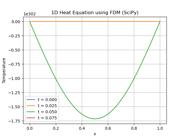
Below is the output of the Heat Equation implementation with the help of FDM using Scipy −

 SparseEfficiencyWarning: spsolve requires A be CSC or CSR matrix format
  u = spsolve(A, b)

Method of Lines (MOL)

The Method of Lines (MOL) is a numerical technique used to solve Partial Differential Equations (PDEs) by discretizing only the spatial variables by converting the PDE into a system of Ordinary Differential Equations (ODEs). These ODEs can then be solved using standard ODE solvers over the time variable. The advantage of MOL is that it separates the spatial and temporal components by allowing the use of efficient ODE techniques for time evolution.

Steps of MOL

Here are the steps of implementing the MOL using the scipy library −

• Spatial Discretization: Discretize the spatial dimension(s) using methods such as finite differences, finite volumes or finite elements.
• Formulation of ODEs: Once the spatial derivatives are discretized, the PDE turns into a system of ODEs with respect to time.
• Time Integration: Use standard ODE solvers such as Runge-Kutta, implicit methods to solve the system of ODEs in time.

Solving the Heat Equation using MOL

The 2D Heat Equation is an extension of the 1D heat equation to two spatial dimensions. It is represented as follows −

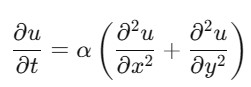
where (,,) is the temperature distribution, is the thermal diffusivity and and are the spatial variables.

Following is the code of implementing the 2d Heat equation using the SciPy library MOL method −

import numpy as np
import matplotlib.pyplot as plt
from scipy.integrate import solve_ivp

# Parameters
alpha = 0.01    # Thermal diffusivity
Lx, Ly = 1.0, 1.0  # Dimensions of the 2D domain
nx, ny = 50, 50    # Number of spatial grid points
dx, dy = Lx / (nx - 1), Ly / (ny - 1)  # Spatial step sizes
x = np.linspace(0, Lx, nx)
y = np.linspace(0, Ly, ny)

# Create a meshgrid for 2D domain
X, Y = np.meshgrid(x, y)

# Initial condition: Gaussian distribution at the center
u_initial = np.exp(-100 * ((X - 0.5)**2 + (Y - 0.5)**2)).flatten()

# Function to compute the right-hand side of the ODE system
def heat_equation_2d(t, u):
    u = u.reshape((nx, ny))  # Reshape to 2D
    dudx2 = np.zeros_like(u)
    dudy2 = np.zeros_like(u)

    # Compute second derivatives using finite differences
    dudx2[1:-1, :] = (u[2:, :] - 2 * u[1:-1, :] + u[:-2, :]) / dx**2
    dudy2[:, 1:-1] = (u[:, 2:] - 2 * u[:, 1:-1] + u[:, :-2]) / dy**2

    # Return the result as a flattened array
    return (alpha * (dudx2 + dudy2)).flatten()

# Time points for the solution
t_span = (0, 0.05)  # Time interval
t_eval = np.linspace(0, 0.05, 200)  # Time evaluation points

# Solve the system of ODEs using solve_ivp
sol = solve_ivp(heat_equation_2d, t_span, u_initial, method='RK45', t_eval=t_eval)

# Plot the solution at different time steps
for i in range(0, len(sol.t), 50):
    plt.figure()
    u_plot = sol.y[:, i].reshape((nx, ny))
    plt.contourf(X, Y, u_plot, 20, cmap='hot')
    plt.colorbar(label='Temperature')
    plt.title(f'Temperature Distribution at t = {sol.t[i]:.3f}')
    plt.xlabel('x')
    plt.ylabel('y')
    plt.show()

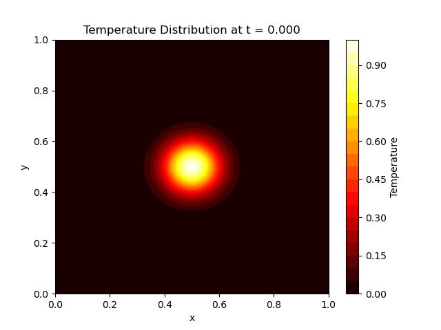
Here is the output of the 2d Heat Equation implementation with the help of MOL using SciPy −

Spectral Methods

Spectral methods are a class of numerical techniques used to solve differential equations by transforming them into a spectral space i.e., frequency domain. These methods involve expanding the solution to a problem in terms of a set of basis functions, typically trigonometric polynomials i.e., Fourier series) or orthogonal polynomials i.e., Chebyshev or Legendre polynomials. They are particularly powerful for problems defined on bounded domains and are known for their high accuracy with fewer grid points compared to finite difference methods.

Key Characteristics of Spectral Methods

Below are the key characteristics of Spectral Methods in SciPy −

• High Accuracy: Spectral methods typically exhibit exponential convergence rates for smooth problems by making them very efficient for achieving high accuracy with fewer degrees of freedom.
• Global Basis Functions: Unlike local methods such as finite differences, spectral methods use global basis functions that span the entire domain by allowing for smooth approximations of the solution.
• Efficiency: They are particularly efficient for problems where the solution is smooth, as they require fewer grid points to achieve a desired accuracy compared to local methods.
• Complexity: Implementing spectral methods can be complex especially in higher dimensions or for non-linear problems.

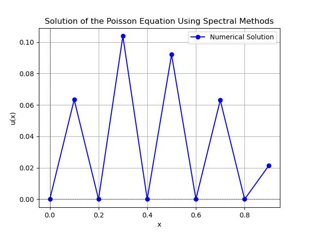
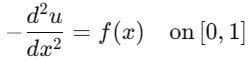
Solving a BVP Using Spectral Methods

Here is the example of solving the one dimensional Poisson equation using the spectral methods in SciPy. The Poisson equation can be given as −

import numpy as np
import matplotlib.pyplot as plt
from scipy.linalg import solve

# Domain and parameters
L = 1.0         # Length of the domain
N = 10          # Number of grid points (Fourier modes)
x = np.linspace(0, L, N + 1)  # Grid points (including boundary)
x = x[:-1]      # Remove the last point to avoid duplication (periodicity)

# Define the Fourier wave numbers (k), avoiding k=0 for singularity issues
k = np.fft.fftfreq(N, d=(x[1] - x[0])) * 2 * np.pi
k = k[1:]  # Remove the k=0 mode to avoid singularity

# Define the right-hand side function f(x) = -2 for the Poisson equation
f = -2 * np.ones(N - 1)  # Exclude the boundary points for solving the internal domain

# Construct the matrix A for the Poisson equation in Fourier space
A = -np.diag(k**2)

# Solve the system Au = f
u_hat = solve(A, f)

# Calculate the solution in physical space using the inverse Fourier transform
u = np.zeros_like(x)
for n in range(N - 1):
    u += u_hat[n] * np.sin((n + 1) * np.pi * x / L)

# Apply boundary conditions (since u(0) = 0 and u(L) = 0, no further adjustment needed)

# Plot the numerical solution
plt.plot(x, u, label='Numerical Solution', color='blue', marker='o')
plt.title('Solution of the Poisson Equation Using Spectral Methods')
plt.xlabel('x')
plt.ylabel('u(x)')
plt.axhline(0, color='black', lw=0.5, ls='--')
plt.axvline(0, color='black', lw=0.5, ls='--')
plt.grid(True)
plt.legend()
plt.show()

Following is the output of the Poisson Equation output

Finite Element Method (FEM)

The Finite Element Method (FEM) is a powerful numerical technique for solving partial differential equations (PDEs) by breaking down a complex problem domain into smaller, simpler subdomains called elements. Within these elements the solution is approximated by simpler functions, typically polynomials. FEM is widely used for structural analysis, heat transfer, fluid dynamics and other engineering applications.

Key steps in the FEM process include

• Discretization: Dividing the domain into finite elements such as triangles, quadrilaterals, etc.
• Shape Functions: Approximating the solution within each element using shape functions.
• Assembly: Combining the local solutions from each element to form a global system of equations.
• Solving: Solving the resulting system of algebraic equations for the nodal values.
• Post-Processing: Interpreting the results for the entire domain.

Solving 1D FEM for a Simple Boundary Value

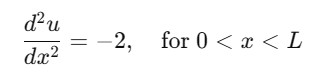
Consider solving the one-dimensional Poisson equation as follows −

with boundary conditions (0) = (1) = 0.

Below is the code to implement the poisson equation with help of FEM method in scipy −

import numpy as np
import matplotlib.pyplot as plt
from scipy.sparse import lil_matrix
from scipy.sparse.linalg import spsolve

# Define the number of elements and domain
n_elements = 10
x = np.linspace(0, 1, n_elements + 1)
h = x[1] - x[0]  # Element length

# Define the load function f(x)
def f(x):
    return 1  # Example: constant load function

# Initialize the global stiffness matrix and load vector
K = lil_matrix((n_elements + 1, n_elements + 1))
F = np.zeros(n_elements + 1)

# Assemble the global stiffness matrix and load vector
for i in range(n_elements):
    K[i, i] += 1 / h
    K[i, i + 1] += -1 / h
    K[i + 1, i] += -1 / h
    K[i + 1, i + 1] += 1 / h
    
    # Compute the load vector for the element
    F[i] += f(x[i]) * h / 2
    F[i + 1] += f(x[i + 1]) * h / 2

# Apply boundary conditions (u(0) = u(1) = 0)
K = K[1:-1, 1:-1]
F = F[1:-1]

# Solve the system
u = spsolve(K, F)

# Add boundary values (u(0) = 0 and u(1) = 0)
u = np.concatenate(([0], u, [0]))

# Plot the solution
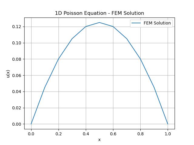
plt.plot(x, u, label='FEM Solution')
plt.xlabel('x')
plt.ylabel('u(x)')
plt.title('1D Poisson Equation - FEM Solution')
plt.grid(True)
plt.legend()
plt.show()

Here is the output of the Poisson Equation using FEM method in scipy −

SparseEfficiencyWarning: spsolve requires A be CSC or CSR matrix format
  u = spsolve(K, F)