SciPy - Polynomial 1-D Interpolation

---

---

Polynomial 1-D Interpolation is a method used to estimate new data points within the range of a set of known data points by fitting a polynomial function through them. In this process a polynomial of degree -1 is constructed that passes through given points. This polynomial can then be used to predict values for intermediate points.

Polynomial interpolation is widely used in numerical analysis and scientific computing for approximating smooth functions. However, high-degree polynomials can lead to inaccuracies due to oscillations near the boundaries and this phenomenon is called as Runge's phenomenon. SciPy provides tools for polynomial interpolation including BarycentricInterpolator and KroghInterpolator which are numerically stable methods for performing this type of interpolation.

Key Characteristics of Polynomial 1-D Interpolation

Following are the key characteristics of polynomial 1-D Interpolation in scipy −

• Degree of Polynomial: A polynomial of degree -1 is fitted through data points.
• Exact Fit to Data: The polynomial passes through all the provided data points exactly.
• Smoothness: The interpolating polynomial is smooth and continuous across its range by making it suitable for approximating smooth functions.
• Runge's Phenomenon: For higher-degree polynomials the oscillations may occur especially near the edges of the interpolation range with reducing accuracy.
• Global Nature: Polynomial interpolation is a global method which change in any data point affects the entire interpolating polynomial.
• Versatility: The polynomial 1-D Interpolation works well for small to medium datasets but may struggle with large datasets due to overfitting or instability.
• Efficient for Small Intervals: This method works well over short intervals where lower-degree polynomials provide good approximations.
• Error Sensitivity: Errors from noisy data points can propagate and affect the entire polynomial by making it sensitive to data precision.

What is Polynomial Degree?

The polynomial degree refers to the highest exponent of the variable in a polynomial expression. It determines the shape and complexity of the polynomial function. The degree of a polynomial is defined as the largest integer such that the polynomial can be expressed in the form as given below −

anxn+an1xn1++a1x+a0, where an, an1,...,a0 are coefficients and n0.

Types of Polynomials by Degree

Polynomials can be classified according to their degree which is defined as the highest power of the variable present in the polynomial expression. Each category of polynomial displays unique characteristics and behaviors by making them appropriate for different mathematical applications and modeling situations. Here are the types of polynomials by degree −

Degree	Name	Description	General Form	Example
0	Constant Polynomial	Outputs a constant value regardless of the input variable x.	p(x) = c	p(x) = 5
1	Linear Polynomial	Describes a straight line defined by a slope and a y-intercept.	p(x) = ax + b	p(x) = 2x + 3
2	Quadratic Polynomial	Forms a parabolic shape with a maximum or minimum point (the vertex).	p(x) = ax + bx + c	p(x) = 3x - 2x + 1
3	Cubic Polynomial	Can have two turning points and cross the x-axis up to three times.	p(x) = ax + bx + cx + d	p(x) = x + 2x - 3x + 4
4	Quartic Polynomial	Can exhibit three turning points and intersect the x-axis up to four times.	p(x) = ax + bx + cx + dx + e	p(x) = 2x - 3x + x + 1
5	Quintic Polynomial	Exhibits complex behavior by allowing for up to four turning points and five x-axis crossings.	p(x) = ax + bx + cx + dx + ex + f	p(x) = x - 2x + x - 1
6	Sextic Polynomial	Higher degree can exhibit more complex oscillations and multiple intersections with the x-axis.	p(x) = ax + bx + cx + dx + ex + fx + g	p(x) = 4x + 3x - x + 7
n	nth Degree Polynomial	Polynomials of degree n can display diverse behaviors based on the coefficients involved.	p(x) = ax + bx + ... + k	Varies based on n

Example

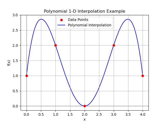
Here's a simple example of 1-D polynomial interpolation using the BarycentricInterpolator from the SciPy library. This example shows how to interpolate a set of known data points with a polynomial and visualize the results −

import numpy as np
import matplotlib.pyplot as plt
from scipy.interpolate import BarycentricInterpolator

# Step 1: Define known data points
# Known x values
x = np.array([0, 1, 2, 3, 4])
# Known y values (e.g., some function values)
y = np.array([1, 2, 0, 2, 1])

# Step 2: Create the polynomial interpolator
interpolator = BarycentricInterpolator(x, y)

# Generate new x values for interpolation
x_new = np.linspace(0, 4, 100)

# Interpolate the y values at new x values
y_new = interpolator(x_new)

# Step 3: Plot the original data points and the polynomial interpolation
plt.scatter(x, y, color='red', label='Data Points', zorder=5)
plt.plot(x_new, y_new, label='Polynomial Interpolation', color='blue', zorder=1)

# Adding labels and title
plt.title('Polynomial 1-D Interpolation Example')
plt.xlabel('x')
plt.ylabel('f(x)')
plt.axhline(0, color='black', lw=0.5, ls='--')
plt.axvline(0, color='black', lw=0.5, ls='--')
plt.grid(True)
plt.legend()
plt.show()

Following is the output of the 1-D polynomial interpolation −

Scipy Functions for Polynomial Interpolation

In SciPy polynomial interpolation is primarily facilitated through the scipy.interpolate module which provides several classes and functions to perform polynomial interpolation in one dimension (1-D). Let's see the key functions and classes related to polynomial interpolation in detail −

Barycentric interpolation

Barycentric interpolation is an efficient method for polynomial interpolation that reduces the computational cost associated with evaluating interpolating polynomials at various points. In SciPy Barycentric interpolation can be performed using the BarycentricInterpolator() function.

Key Features of Barycentric Interpolation

Here are the key features of Barycentric Interpolation class in scipy −

• Efficiency: Barycentric interpolation is computationally efficient for evaluating polynomials especially for large datasets.
• Stability: It is numerically stable by reducing the risk of errors due to ill-conditioned polynomial interpolation.
• Weight Calculation: This method involves calculating weights based on the interpolation points by allowing for fast evaluation of the polynomial at any given point.

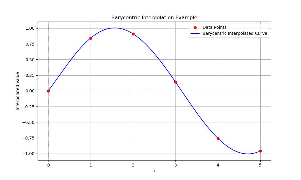
Following is the example of generating the Polynomial Interpolation by using the BarycentricInterpolator() function in scipy −

import numpy as np
import matplotlib.pyplot as plt
from scipy.interpolate import BarycentricInterpolator

# Define the sample data points
x = np.array([0, 1, 2, 3, 4, 5])
y = np.sin(x)  # Function values at the sample points

# Create the Barycentric Interpolator
interpolator = BarycentricInterpolator(x, y)

# Define new x values for interpolation
x_new = np.linspace(0, 5, 100)
y_new = interpolator(x_new)

# Plot the results
plt.figure(figsize=(10, 6))
plt.scatter(x, y, color='red', label='Data Points', zorder=5)
plt.plot(x_new, y_new, label='Barycentric Interpolated Curve', color='blue')
plt.title('Barycentric Interpolation Example')
plt.xlabel('x')
plt.ylabel('Interpolated Value')
plt.axhline(0, color='black', lw=0.5, ls='--')
plt.axvline(0, color='black', lw=0.5, ls='--')
plt.grid()
plt.legend()
plt.show()

Here is the output of the Barycentric Polynomial Interpolation −

Krogh interpolation

Krogh interpolation is a method for polynomial interpolation that allows for the specification of function values and their derivatives at given points. This technique is particularly useful when the data points contain not only function values but also information about the rates of change (derivatives) at those points. Krogh interpolation can provide a more accurate polynomial representation of the underlying function compared to standard polynomial interpolation especially when the derivatives at the interpolation points are known.

Key Features of Krogh Interpolation

Following are the key features of Krogh Interpolation class in scipy −

• Higher Accuracy: By including derivatives the Krogh interpolation can yield more accurate results compared to traditional polynomial interpolation methods particularly for smooth functions.
• Polynomial Degree: The degree of the interpolating polynomial is determined by the total number of points used including both function values and derivative values. This can result in polynomials of varying degrees depending on the number of constraints applied.
• Efficient Calculation: Krogh interpolation uses divided differences to calculate the coefficients of the polynomial by making it computationally efficient.

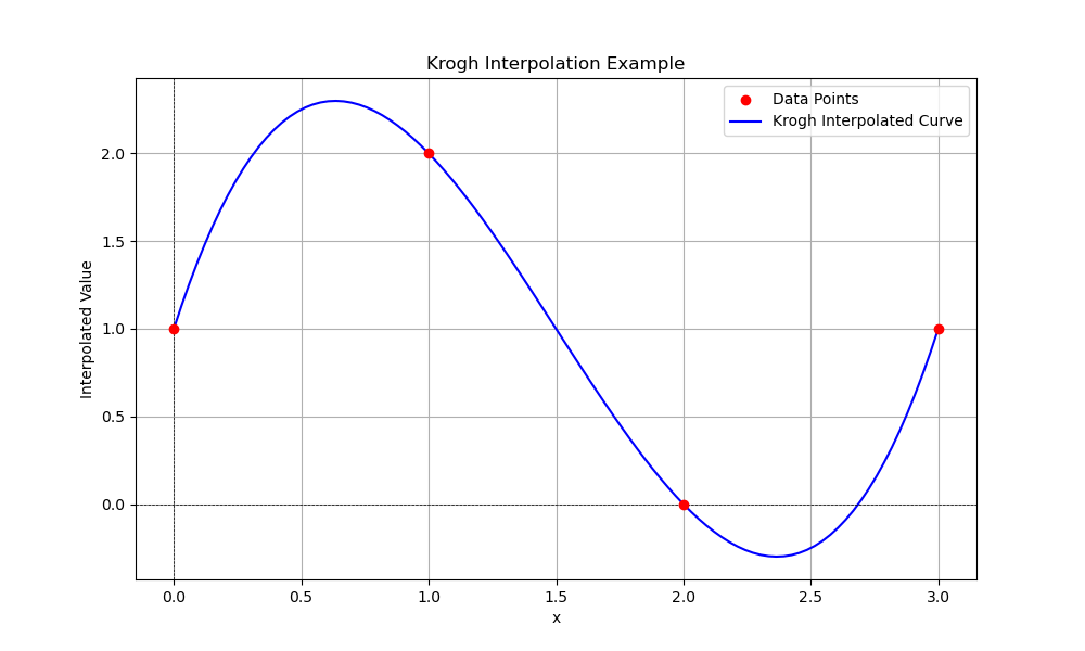
Following is the example of generating the Polynomial Interpolation by using the KroghInterpolator() function in scipy −

import numpy as np
import matplotlib.pyplot as plt
from scipy.interpolate import KroghInterpolator

# Define sample data points (x) and their corresponding function values (y)
x = np.array([0, 1, 2, 3])
y = np.array([1, 2, 0, 1])  # Function values

# Create the Krogh Interpolator (without derivatives)
interpolator = KroghInterpolator(x, y)

# Define new x values for interpolation
x_new = np.linspace(0, 3, 100)
y_new = interpolator(x_new)

# Plot the results
plt.figure(figsize=(10, 6))
plt.scatter(x, y, color='red', label='Data Points', zorder=5)
plt.plot(x_new, y_new, label='Krogh Interpolated Curve', color='blue')
plt.title('Krogh Interpolation Example')
plt.xlabel('x')
plt.ylabel('Interpolated Value')
plt.axhline(0, color='black', lw=0.5, ls='--')
plt.axvline(0, color='black', lw=0.5, ls='--')
plt.grid()
plt.legend()
plt.show()

Below is the output of the Krogh Polynomial Interpolation −

Limitations of Polynomial Interpolation

Here are the limitations of polynomial Interpolation in scipy −

• Runge's Phenomenon: High-degree polynomials can exhibit large oscillations, especially at the edges of the interpolation range by leading to poor approximations.
• Overfitting: A polynomial that is too high in degree can overfit the data by resulting in poor generalization to points outside the known range.
• Computational Complexity: Higher-degree polynomials increase the computational cost and complexity particularly for large datasets.