SciPy Radial Basis Function(RBF) Multi-Dimensional Interpolation

---

---

Radial Basis Function (RBF) interpolation is a method for estimating values at unmeasured points based on a set of known data points. It uses radial basis functions which are real-valued functions whose value depends only on the distance from a center point. This method is particularly effective for scattered data in multiple dimensions.

The Mathematical Formula for Radial Basis Function f(x) can be given as follows −

• N is the number of data points.
• x is the input point where the function value is estimated.
• x_i are the known data points.
• w_i are the weights determined by the values of the function at the data points.
• is a radial basis function which typically depends on the Euclidean distance ||x-x_i||.

Common Radial Basis Functions (RBFs)

Radial Basis Functions are mathematical functions whose value depends only on the distance from a central point. They are widely used in interpolation, machine learning and various numerical methods due to their ability to approximate complex surfaces. Here are some of the most common types of radial basis functions −

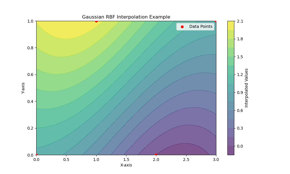
Gaussian RBF

The Gaussian RBF is one of the most widely used radial basis functions. It decreases rapidly as the distance r from the center increases by providing a smooth and localized influence.

Following are the key characteristics of Gaussian RBF −

• Smoothness: The Gaussian function is infinitely differentiable by making it very smooth. This property is beneficial for various applications in interpolation and approximation.
• Local Influence: The effect of a Gaussian RBF diminishes quickly as we move away from the center which means it has a strong local influence which is useful for capturing local variations in data.
• Radial Symmetry: The output only depends on the distance from the center, not the direction by making it rotationally symmetric.
• Applications: Gaussian RBFs are commonly used in various fields as mentioned below −
• Machine Learning: In support vector machines and kernelized methods.
• Data Interpolation: To construct smooth surfaces from scattered data points.
• Function Approximation: For approximating complex functions using RBF networks.

Example

In SciPy we can use the RBFInterpolator for interpolation using the Gaussian RBF. Here is a simple example of how to use the Gaussian RBF in SciPy for 2D interpolation −

import numpy as np
import matplotlib.pyplot as plt
from scipy.interpolate import RBFInterpolator

# Sample data points
x = np.array([0, 1, 2, 3])
y = np.array([0, 1, 0, 1])
z = np.array([1, 2, 0, 1])  # Function values at the points

# Create the RBF interpolator with Gaussian function and specified epsilon
epsilon = 0.5  # Adjust epsilon for smoother or sharper interpolation
interpolator = RBFInterpolator(np.array(list(zip(x, y))), z, kernel='gaussian', epsilon=epsilon)

# Define new points for interpolation
xi, yi = np.meshgrid(np.linspace(0, 3, 100), np.linspace(0, 1, 100))
zi = interpolator(np.array(list(zip(xi.ravel(), yi.ravel())))).reshape(xi.shape)

# Plot the results
plt.figure(figsize=(10, 6))
plt.scatter(x, y, c='red', label='Data Points', zorder=5)
plt.contourf(xi, yi, zi, levels=15, cmap='viridis', alpha=0.7)
plt.colorbar(label='Interpolated Values')
plt.title('Gaussian RBF Interpolation Example')
plt.xlabel('X-axis')
plt.ylabel('Y-axis')
plt.legend()
plt.show()

Here is the output of the Gaussian RBF interpolation in scipy −

Multiquadric RBF

The Multiquadric Radial Basis Function (RBF) is a type of radial basis function that is widely used for interpolation which particularly in scattered data interpolation and surface fitting. It is defined mathematically by the following formula −

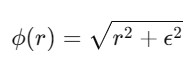
Where −

• r is the Euclidean distance between a given point and a center point.
• is a shape parameter i.e., positive constant which controls the "flatness" or spread of the function.

Here are the key Features of Multiquadric RBF −

• Global Influence: Unlike some other RBFs like the Gaussian, the multiquadric RBF tends to have a global smoothing effect, meaning that a change at one point can influence distant points.
• Flexibility: The shape parameter can be adjusted to control how rapidly the function decays by allowing for control over the balance between local and global influences.
• Smooth Interpolation: It generally produces a smooth interpolation, which makes it useful for modeling surfaces or functions that are expected to be continuous and differentiable.
• Applications: Multiquadric RBFs are commonly used in various fields as mentioned below −
• Surface fitting in 2D or 3D.
• Geospatial data interpolation such as terrain modeling.
• Solving partial differential equations(PDEs) via mesh-free methods.

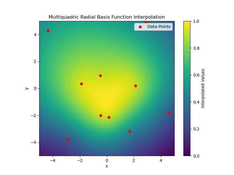
Example

This example shows how to generate a smooth surface based on the scattered data points using the multiquadric RBF −

import numpy as np
import matplotlib.pyplot as plt
from scipy.interpolate import Rbf

# Define sample data points
x = np.random.uniform(-5, 5, 10)  # 10 random x values
y = np.random.uniform(-5, 5, 10)  # 10 random y values
z = np.sin(np.sqrt(x**2 + y**2))  # Function values at the points

# Create a multiquadric RBF interpolator
rbf_interpolator = Rbf(x, y, z, function='multiquadric', epsilon=1)

# Create a grid to interpolate
x_grid, y_grid = np.linspace(-5, 5, 100), np.linspace(-5, 5, 100)
x_grid, y_grid = np.meshgrid(x_grid, y_grid)

# Apply the RBF interpolator to the grid
z_grid = rbf_interpolator(x_grid, y_grid)

# Plot the results
plt.figure(figsize=(8, 6))
plt.imshow(z_grid, extent=(-5, 5, -5, 5), origin='lower', cmap='viridis')
plt.scatter(x, y, color='red', label='Data Points')
plt.colorbar(label='Interpolated Values')
plt.title('Multiquadric Radial Basis Function Interpolation')
plt.xlabel('x')
plt.ylabel('y')
plt.legend()
plt.show()

Here is the output of the Multiquadric RBF interpolation in scipy −

Inverse Multiquadric RBF

The Inverse Multiquadric Radial Basis Function(RBF) is a type of radial basis function used for interpolation and machine learning tasks particularly in multivariate interpolation. The mathematical formula of Inverse Multiquadric RBF is given as follows −

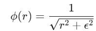
Where −

• r is the Euclidean distance between points.
• is a shape parameter that controls the smoothness and spread of the function.

Here are the key characteristics of Inverse Multiquadric RBF −

• Local Influence: The inverse multiquadric has a pronounced local effect, meaning it gives higher importance to closer points.
• Smoothness: It produces a smooth interpolation surface.
• Shape Parameter: The value of significantly affects the function. A small leads to sharp peaks around the interpolation points, while a larger results in smoother and broader shapes.
• Applications: It is commonly used in spatial interpolation, particularly in scattered data fitting.

Example

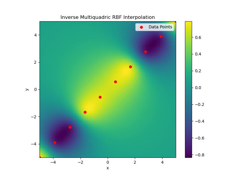
Following is an example which shows how to generate the Inverse multiquadric RBF Interpolation in scipy −

import numpy as np
import matplotlib.pyplot as plt
from scipy.interpolate import Rbf

# Create some sample data points
x = np.linspace(-5, 5, 10)  # x-coordinates
y = np.linspace(-5, 5, 10)  # y-coordinates
z = np.sin(np.sqrt(x**2 + y**2))  # Sample function values at the points

# Create a meshgrid for interpolation
xi = np.linspace(-5, 5, 100)  # Fine grid for x
yi = np.linspace(-5, 5, 100)  # Fine grid for y
xi, yi = np.meshgrid(xi, yi)   # Create 2D grid

# Apply the Inverse Multiquadric RBF for interpolation
rbf = Rbf(x, y, z, function='inverse_multiquadric', epsilon=1)
zi = rbf(xi, yi)  # Interpolated values

# Plot the results
plt.figure(figsize=(8, 6))
plt.imshow(zi, extent=(-5, 5, -5, 5), origin='lower', cmap='viridis')
plt.colorbar()
plt.scatter(x, y, color='red', label='Data Points')
plt.title('Inverse Multiquadric RBF Interpolation')
plt.xlabel('x')
plt.ylabel('y')
plt.legend()
plt.show()

Here is the output of the Inverse Multiquadric RBF interpolation in scipy −

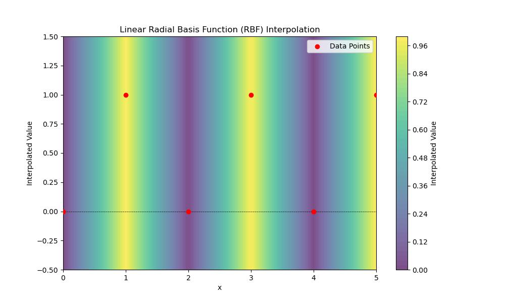
Linear RBF

The Linear Radial Basis Function(RBF) is one of the simplest RBFs with a direct relationship between the distance and the function value. The linear RBF provides a basic approach but lacks the flexibility of more complex functions such as Gaussian or cubic RBFs which are better suited for smoothing and interpolation tasks. Following is the Mathematical representation of the Linear RBF −

(r) = r

Where r is the Euclidean distance between a data point and the center.

Below are the key characteristics of Linear RBF −

• Behavior: This function grows linearly with distance which means it doesn't provide any smoothing beyond the linear scaling. It is not commonly used for practical interpolation tasks that require smoothness or local influence.
• Application: It may be used in simple or low-dimensional problems but is less effective for complex, noisy or high-dimensional data.

Example

This example shows how to create a grid of points, assign values to some of these points and then interpolate values at new points using the Linear RBF −

import numpy as np
import matplotlib.pyplot as plt
from scipy.interpolate import RBFInterpolator

# Sample data points (x, y) and their corresponding values (z)
x = np.array([0, 1, 2, 3, 4, 5])
y = np.array([0, 1, 0, 1, 0, 1])  # Function values at the points

# Create a grid of points for interpolation
grid_x, grid_y = np.meshgrid(np.linspace(0, 5, 100), np.linspace(-0.5, 1.5, 100))

# Create the RBF interpolator using linear basis function
rbf = RBFInterpolator(x.reshape(-1, 1), y, kernel='linear')

# Perform interpolation on the grid points
# Here we only need to use the x-values, y is just for the grid
grid_points = grid_x.ravel()  # Flatten the grid for RBF interpolator
interpolated_values = rbf(grid_points.reshape(-1, 1))  # Reshape for RBFInterpolator

# Reshape the interpolated values to match the grid shape
interpolated_values = interpolated_values.reshape(grid_x.shape)

# Plotting
plt.figure(figsize=(10, 6))
plt.scatter(x, y, color='red', label='Data Points', zorder=5)
plt.contourf(grid_x, grid_y, interpolated_values, levels=50, cmap='viridis', alpha=0.7)
plt.colorbar(label='Interpolated Value')
plt.title('Linear Radial Basis Function (RBF) Interpolation')
plt.xlabel('x')
plt.ylabel('Interpolated Value')
plt.axhline(0, color='black', lw=0.5, ls='--')
plt.axvline(0, color='black', lw=0.5, ls='--')
plt.legend()
plt.show()

Below is the output of the Linear RBF interpolation in scipy −

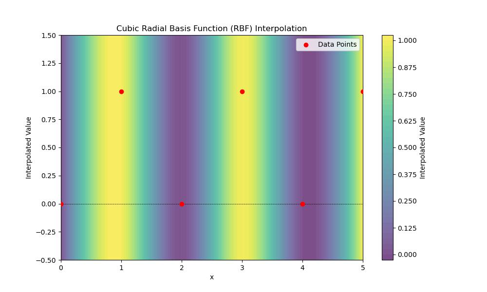
Cubic RBF

Cubic Radial Basis Function (RBF) interpolation is a method used to interpolate data in multiple dimensions using cubic radial basis functions. In this approach the interpolating function is constructed as a linear combination of cubic RBFs centered at the data points. Below is the Mathematical representation of the Cubic RBF −

(r) = r3

Where r is the Euclidean distance between a point x and a center c i.e., r=xc).

Following are the key characteristics of Cubic RBF −

• Smoothness: The cubic RBF is a smooth function and provides smooth interpolation results by making it suitable for approximating continuous data.
• Global influence: Each RBF influences all points in the domain which can result in a smooth overall shape.
• Shape flexibility: The cubic form allows for flexible fitting to various types of data.

Example

We can perform cubic Radial Basis Function (RBF) interpolation using scipy by specifying the kernel as cubic when creating the RBFInterpolator. Below is an example that shows how to implement cubic RBF interpolation −

import numpy as np
import matplotlib.pyplot as plt
from scipy.interpolate import RBFInterpolator

# Sample data points (x, y) and their corresponding values (z)
x = np.array([0, 1, 2, 3, 4, 5])
y = np.array([0, 1, 0, 1, 0, 1])  # Function values at the points

# Create a grid of points for interpolation
grid_x = np.linspace(0, 5, 100)
grid_y = np.linspace(-0.5, 1.5, 100)
grid_x, grid_y = np.meshgrid(grid_x, grid_y)

# Create the RBF interpolator using cubic basis function
rbf = RBFInterpolator(x.reshape(-1, 1), y, kernel='cubic')

# Perform interpolation on the grid points
interpolated_values = rbf(grid_x.ravel().reshape(-1, 1))

# Reshape the interpolated values to match the grid shape
interpolated_values = interpolated_values.reshape(grid_x.shape)

# Plotting
plt.figure(figsize=(10, 6))
plt.scatter(x, y, color='red', label='Data Points', zorder=5)
plt.contourf(grid_x, grid_y, interpolated_values, levels=50, cmap='viridis', alpha=0.7)
plt.colorbar(label='Interpolated Value')
plt.title('Cubic Radial Basis Function (RBF) Interpolation')
plt.xlabel('x')
plt.ylabel('Interpolated Value')
plt.axhline(0, color='black', lw=0.5, ls='--')
plt.axvline(0, color='black', lw=0.5, ls='--')
plt.legend()
plt.show()

Below is the output of the c RBF interpolation in scipy −

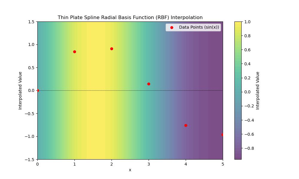
Thin Plate Spline RBF

Thin Plate Spline (TPS) Radial Basis Function (RBF) is a specific type of radial basis function used in interpolation especially when the data points lie in multi-dimensional space. Below is the Mathematical representation of the Thin Plate Spline RBF −

(r) = r2log(r)

Where r is the Euclidean distance between a point x and a center c i.e., r=xx_i).

Following are the key characteristics of Thin Plate Spline RBF −

• Smoothness: TPS is known for producing very smooth interpolating surfaces by making it ideal for applications where smoothness of the resulting surface is critical.
• Global influence: Unlike some other radial basis functions such as Gaussian then the influence of TPS decays more slowly with distance which means that each data point has a global impact on the resulting interpolation.
• Dimensionality: It works well for interpolating data in higher dimensions such as 2D or 3D by making it popular in image warping, surface fitting and geographic data applications.

Example

Here is an example of how to implement Radial Basis Function (RBF) interpolation using the thin plate spline kernel with RBFInterpolator in SciPy −

import numpy as np
import matplotlib.pyplot as plt
from scipy.interpolate import RBFInterpolator

# Define sample data points (xi, yi) and their corresponding values
x = np.array([0, 1, 2, 3, 4, 5])        # x-coordinates of data points
y = np.sin(x)                           # Corresponding y-values (sine function)

# Create a grid of points for interpolation
grid_x = np.linspace(0, 5, 100)         # x values for the grid
grid_y = np.linspace(-1.5, 1.5, 100)    # y values for the grid
grid_x, grid_y = np.meshgrid(grid_x, grid_y)

# Create the RBF interpolator using Thin Plate Spline kernel
rbf = RBFInterpolator(x.reshape(-1, 1), y, kernel='thin_plate_spline')

# Prepare the grid points for interpolation
grid_points = np.column_stack((grid_x.ravel(), grid_y.ravel()))

# Perform interpolation on the grid points
# Use both x and y coordinates for the input; we will ignore y values in the interpolation
interpolated_values = rbf(grid_points[:, 0].reshape(-1, 1))  # Reshape to 2D

# Reshape the interpolated values to match the grid shape
interpolated_values = interpolated_values.reshape(grid_x.shape)

# Plotting
plt.figure(figsize=(10, 6))
plt.scatter(x, y, color='red', label='Data Points (sin(x))', zorder=5)
plt.contourf(grid_x, grid_y, interpolated_values, levels=50, cmap='viridis', alpha=0.7)
plt.colorbar(label='Interpolated Value')
plt.title('Thin Plate Spline Radial Basis Function (RBF) Interpolation')
plt.xlabel('x')
plt.ylabel('Interpolated Value')
plt.axhline(0, color='black', lw=0.5, ls='--')
plt.axvline(0, color='black', lw=0.5, ls='--')
plt.legend()
plt.show()

Below is the output of the Thin plate spline RBF interpolation in scipy −

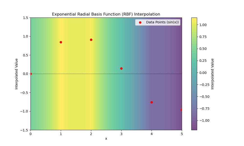
Exponential RBF

Exponential Radial Basis Function (RBF) is a type of radial basis function commonly used in interpolation, machine learning and neural networks. It is defined by its exponential decay which allows it to capture localized variations in data more effectively than other types of RBFs. Below is the Mathematical representation of the Exponential RBF −

(r) = e-r

Where r is the Euclidean distance from the center of the function to a point in the input space which often calculated as r=xx_i) and is a parameter that controls the width of the radial basis function. A larger leads to a more localized response while a smaller results in a smoother and more spread-out response.

Following are the key characteristics of Exponential RBF −

• Localization: The exponential decay allows the function to be localized, meaning it has a stronger influence near its center and rapidly diminishes further away.
• Smoothness: The exponential function is infinitely differentiable by making it a smooth function which is beneficial for interpolation and approximation tasks.
• Applications: It is often used in machine learning algorithms such as support vector machines and in radial basis function networks for function approximation.

Example

This example generates some sample data points and then uses the Exponential RBF to interpolate values between those points −

import numpy as np
import matplotlib.pyplot as plt
from scipy.interpolate import RBFInterpolator

# Define sample data points (xi, yi) and their corresponding values
x = np.array([0, 1, 2, 3, 4, 5])        # x-coordinates of data points
y = np.sin(x)                           # Corresponding y-values (sine function)

# Create a grid of points for interpolation
grid_x = np.linspace(0, 5, 100)         # x values for the grid
grid_y = np.linspace(-1.5, 1.5, 100)    # y values for the grid
grid_x, grid_y = np.meshgrid(grid_x, grid_y)

# Create the RBF interpolator using Exponential kernel
# Note: 'exponential' is not directly available in SciPy, we will use a custom implementation
class ExponentialRBF:
    def __init__(self, centers, values, beta=1.0):
        self.centers = centers
        self.values = values
        self.beta = beta

    def __call__(self, x):
        distances = np.linalg.norm(x[:, np.newaxis] - self.centers, axis=2)  # Compute distances
        return np.dot(np.exp(-self.beta * distances), self.values)  # Apply the exponential RBF

# Initialize the custom RBF interpolator
exponential_rbf = ExponentialRBF(x.reshape(-1, 1), y, beta=1.0)

# Prepare the grid points for interpolation
grid_points = np.column_stack((grid_x.ravel(), grid_y.ravel()))

# Perform interpolation on the grid points using only the x-coordinates
interpolated_values = exponential_rbf(grid_points[:, 0].reshape(-1, 1))

# Reshape the interpolated values to match the grid shape
interpolated_values = interpolated_values.reshape(grid_x.shape)

# Plotting
plt.figure(figsize=(10, 6))
plt.scatter(x, y, color='red', label='Data Points (sin(x))', zorder=5)
plt.contourf(grid_x, grid_y, interpolated_values, levels=50, cmap='viridis', alpha=0.7)
plt.colorbar(label='Interpolated Value')
plt.title('Exponential Radial Basis Function (RBF) Interpolation')
plt.xlabel('x')
plt.ylabel('Interpolated Value')
plt.axhline(0, color='black', lw=0.5, ls='--')
plt.axvline(0, color='black', lw=0.5, ls='--')
plt.legend()
plt.show()

Following is the output of the Exponential RBF interpolation in scipy −