SciPy - Short-Time Fourier Transform (STFT)

---

---

Short-Time Fourier Transform in SciPy

The Short-Time Fourier Transform (STFT) in SciPy is a tool to analyze signals in both the time and frequency domains. It works by dividing a signal into small, overlapping segments by using a sliding window and then performing a Fourier Transform on each segment.

The result is a time-frequency representation of the signal by showing how its frequency content changes over time. Mathematically, the STFT of a signal x(t) is defined as follows −

X(t, f) = - x() w( - t)  e-j 2 f  d

Where −

• x() is the signal
• w(t) is the window function centered at time
• e^j2f represents the Fourier Transform.
• and are the time and frequency variables respectively.

The window function ensures that only a small segment of the signal around contributes to the Fourier Transform at that point.

Steps of STFT

Following are the steps to perform the Short Time Fourier Transform in SciPy −

• Windowing: This divides the signal into overlapping segments using a window function. The window function is typically chosen to minimize spectral leakage e.g., Hann, Hamming, Blackman.
• Fourier Transform: Then apply the Fourier Transform to each windowed segment.
• Time-Frequency Representation: Finally combine the results for all segments to form a 2D representation with time and frequency axes.

Short-Time Fourier Transform (STFT) in SciPy

In SciPy we have the function scipy.signal.stft() to perform the Short-Time Fourier Transform which provides flexibility in parameters such as the window type, segment length, overlap and FFT size.

Syntax

Following is the syntax of scipy.signal.stft() function which is used to perform Short-Time Fourier Transform −

scipy.signal.stft(x,fs=1.0,window='hann',nperseg=256,noverlap=None,nfft=None,detrend=False,return_onesided=True,boundary='zeros',padded=True,axis=-1,scaling='spectrum')

Parameters

Here are the parameters of the function scipy.signal.stft() −

• x(array_like): Input signal. The data to be transformed.
• fs(float, optional): Sampling frequency of the input signal. Default is 1.0.
• window(str or tuple or array_like, optional): Desired window function to apply to each segment. Defaults to 'hann'.
• nperseg(int, optional): Length of each segment for the STFT. Default is 256.
• noverlap(int, optional): Number of points to overlap between segments. If not specified, it defaults to half of nperseg.
• nfft(int, optional): Number of points for the FFT computation. If not provided, defaults to nperseg.
• detrend(str or function or bool, optional): Specifies how to detrend each segment. Default is False (no detrending).
• return_onesided(bool, optional): If True, returns a one-sided spectrum for real signals. Default is True.
• boundary(str or None, optional): Specifies how to handle the signal boundaries. Default is 'zeros'.
• padded(bool, optional): If True, pads each segment to the nearest power of two. Default is True.
• axis(int, optional): Axis along which the STFT is computed. Default is -1 (last axis).
• scaling(str, optional): Determines the scaling of the STFT output. Options are 'spectrum' (default) and 'density'.

Basic Example

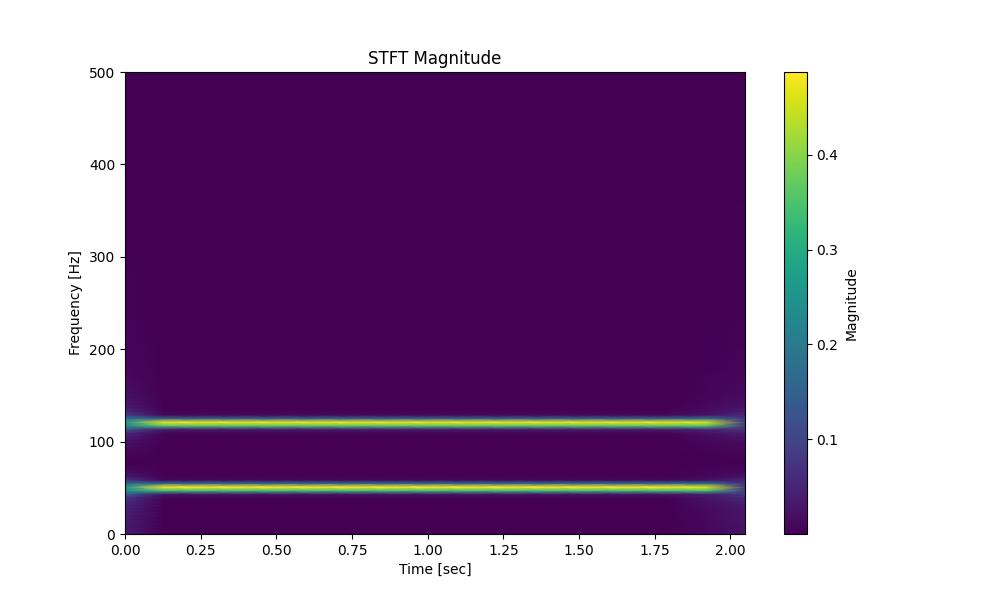
Following is the example which computes and plots the STFT of a signal composed of two sine waves by using the function scipy.signal.stft() with default parameters −

import numpy as np
from scipy.signal import stft
import matplotlib.pyplot as plt

# Create a simple signal
fs = 1000  # Sampling frequency
t = np.linspace(0, 2, 2 * fs, endpoint=False)  # 2-second time vector
x = np.sin(2 * np.pi * 50 * t) + np.sin(2 * np.pi * 120 * t)  # Two sine waves

# Compute the STFT
f, t, Zxx = stft(x, fs=fs, window='hann', nperseg=256, noverlap=128)

# Plot the STFT Magnitude
plt.figure(figsize=(10, 6))
plt.pcolormesh(t, f, np.abs(Zxx), shading='gouraud')
plt.title('STFT Magnitude')
plt.ylabel('Frequency [Hz]')
plt.xlabel('Time [sec]')
plt.colorbar(label='Magnitude')
plt.show()

Below is the output of the STFT basic example −

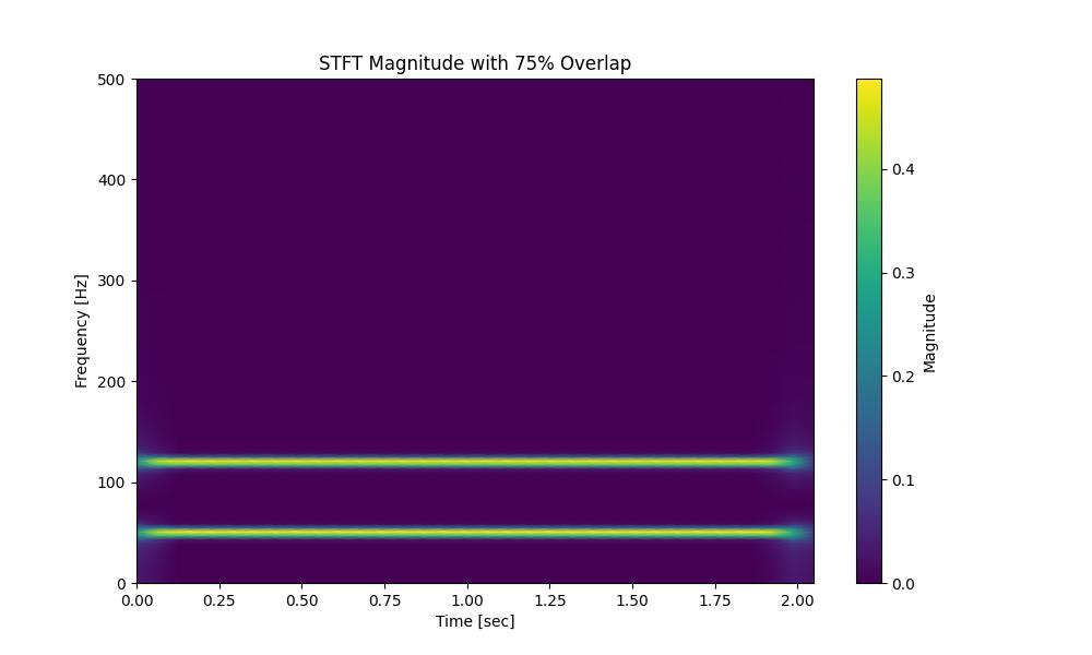
Adjusting Overlap

This example shows how to change the overlap between segments to 75% resulting in smoother time-frequency resolution −

import numpy as np
from scipy.signal import stft
import matplotlib.pyplot as plt

# Create a simple signal
fs = 1000  # Sampling frequency
t = np.linspace(0, 2, 2 * fs, endpoint=False)  # 2-second time vector
x = np.sin(2 * np.pi * 50 * t) + np.sin(2 * np.pi * 120 * t)  # Two sine waves

# Compute the STFT
f, t, Zxx = stft(x, fs=fs, window='hann', nperseg=256, noverlap=128)

# Plot the STFT Magnitude
plt.figure(figsize=(10, 6))
plt.pcolormesh(t, f, np.abs(Zxx), shading='gouraud')
plt.title('STFT Magnitude')
plt.ylabel('Frequency [Hz]')
plt.xlabel('Time [sec]')
plt.colorbar(label='Magnitude')
plt.show()

Below is the output of the STFT which adjusts the overlap using the function scipy.signal.stft() −

Applications of STFT

Here are the applications of SciPy Short Time Fourier Transform −

• Speech and Audio Processing: Analyze time-varying frequency content of speech signals.
• Music Analysis: Identify harmonic components and beats in music.
• Biomedical Signals: Analyze non-stationary signals like EEG or ECG.
• Vibration Analysis: Detect faults in rotating machinery.
• Communications: Demodulate time-varying frequency signals.