SciPy - Spline 1-D Interpolation

---

---

Spline interpolation in SciPy is a technique for creating smooth curves through a set of data points by fitting piecewise polynomials between the points. Splines are particularly cubic splines which are used to interpolate the data in a way that ensures both the function and its derivatives are continuous by providing a smooth and accurate representation of the data.

In SciPy the spline interpolation is implemented in the scipy.interpolate module with functions such as CubicSpline() and InterpolatedUnivariateSpline(). These functions can generate smooth interpolating functions by making them suitable for data fitting and graphical applications.

Key Features of Spline Interpolation

Below are the key features of the Spline Interpolation in Scipy −

• Piecewise Polynomial Fit: Spline interpolation divides the data range into intervals and fits a polynomial to each interval by ensuring a smooth transition between points.
• Continuity of Derivatives: For cubic splines the first and second derivatives are continuous at the boundaries of the intervals (called knots) by providing a smooth curve.
• Flexibility: Splines can be adapted to handle various boundary conditions, such as clamped or natural, giving more control over the behavior of the curve at the ends.
• Accuracy: Compared to higher-degree polynomials the splines are less prone to oscillations by making them more accurate for smoothly interpolating data.
• Efficiency: Spline interpolation is computationally efficient especially for large datasets due to its piecewise nature.
• Applications: Spline interpolation is widely used in data fitting, computer graphics (smooth animations) and engineering simulations where smooth curves are essential.

Advantages of Spline Interpolation

Below are the advantages of using the Spline Interpolation in Scipy −

• Smoothness: Cubic splines provide a smooth curve without the oscillations seen in high-degree polynomial interpolations.
• Local Control: Adjusting one data point will only affect the nearby spline segments, not the entire curve.
• Flexibility: This method can be easily adapted for various boundary conditions.

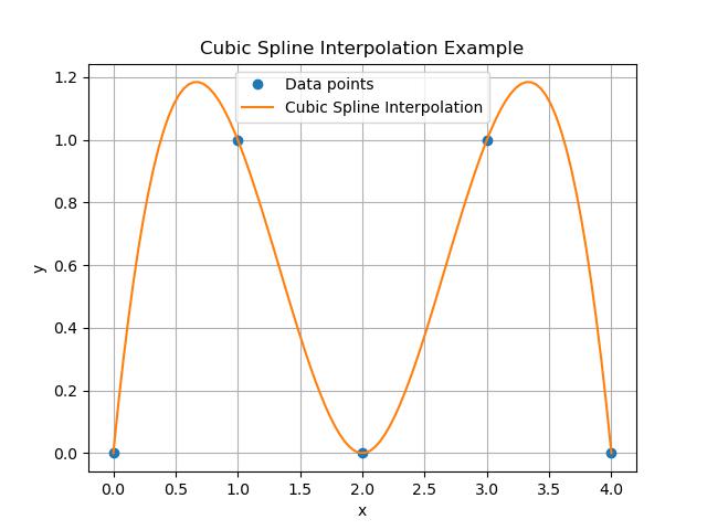
Example

This example shows how to use the spline interpolation in scipy, for smoothly connects the data points −

import numpy as np
import matplotlib.pyplot as plt
from scipy.interpolate import CubicSpline

# Define sample data points (x) and their corresponding function values (y)
x = np.array([0, 1, 2, 3, 4, 5])
y = np.array([0, 1, 0, 1, 0, 1])

# Create a cubic spline interpolator
cs = CubicSpline(x, y)

# Define new x values for interpolation
x_new = np.linspace(0, 5, 100)
y_new = cs(x_new)

# Plot the results
plt.scatter(x, y, color='red', label='Data Points')
plt.plot(x_new, y_new, label='Cubic Spline Interpolated Curve', color='blue')
plt.title('Cubic Spline Interpolation Example')
plt.xlabel('x')
plt.ylabel('Interpolated Value')
plt.axhline(0, color='black', lw=0.5, ls='--')
plt.axvline(0, color='black', lw=0.5, ls='--')
plt.grid(True)
plt.legend()
plt.show()

Following is the output of the simple spline interpolation in scipy −

Functions used for Spline Interpolation

SciPy provides several functions for spline interpolation in which each catering to different types of interpolation needs. These functions are available under the scipy.interpolate module and can handle both 1-D and higher-dimensional spline interpolations. Here's are the key functions in SciPy for spline interpolation −

Function	Purpose	Key Features
CubicSpline	Performs cubic spline interpolation	- Smooth cubic polynomials between points - Supports boundary conditions
splrep and splev	B-spline representation (splrep) and evaluation (splev)	- splrep: Finds B-spline - splev: Evaluates at given points
UnivariateSpline	Univariate spline interpolation of degree k	- Smooth spline - Optional smoothing factor
BSpline	More general B-spline with control over knots and coefficients	- Full control over the spline - Customizable knots and basis functions
make_interp_spline	Constructs a B-spline approximation	- General spline orders - Similar to CubicSpline
PchipInterpolator	Piecewise cubic Hermite interpolation	- Monotonic, piecewise cubic - No overshooting

CubicSpline() Function

The CubicSpline() function in SciPy provides a powerful method for cubic spline interpolation which fits a piecewise cubic polynomial between given data points. A cubic spline ensures smoothness at the data points and the first and second derivatives of the polynomial are continuous across these points. This results in a smooth curve that passes through all data points by making it ideal for interpolation tasks where smoothness is required.

Syntax

Following is the syntax of using the CubicSpline() function in scipy −

scipy.interpolate.CubicSpline(x, y, bc_type='not-a-knot', extrapolate=True)

Parameters

Below are the parameters of the CubicSpline() function in scipy −

• x: 1-D array of independent variable data points.
• y: 1-D array of dependent variable data points.
• bc_type: Boundary condition type with default value as 'not-a-knot and can also be 'natural' or 'clamped'.
• extrapolate: Whether to extrapolate to out-of-bounds points and the default value is True.

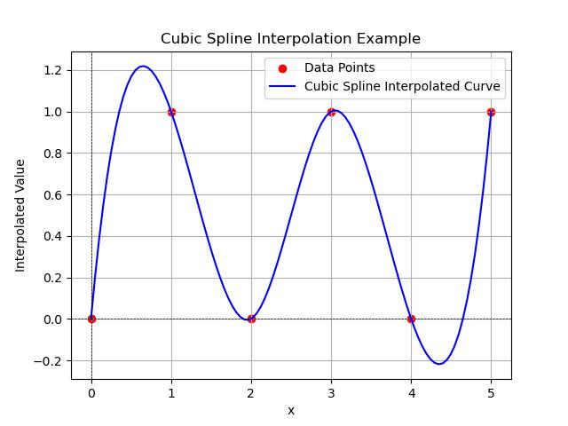
Example

In this example a cubic spline is fit through a set of data points and the resulting smooth curve is plotted. We can also adjust the boundary conditions by modifying the bc_type parameter −

import numpy as np
import matplotlib.pyplot as plt
from scipy.interpolate import CubicSpline

# Define data points
x = np.array([0, 1, 2, 3, 4])
y = np.array([0, 1, 0, 1, 0])

# Perform cubic spline interpolation
cs = CubicSpline(x, y)

# Generate new points for interpolation
x_new = np.linspace(0, 4, 100)
y_new = cs(x_new)

# Plot the results
plt.plot(x, y, 'o', label='Data points')
plt.plot(x_new, y_new, label='Cubic Spline Interpolation')
plt.title('Cubic Spline Interpolation Example')
plt.xlabel('x')
plt.ylabel('y')
plt.grid(True)
plt.legend()
plt.show()

Below is the output of the Cubic Spline Interpolation in Scipy −

splrep() and splev() Functions

In SciPy the splrep and splev are two functions used together for B-spline interpolation. Heres a detailed explanation of each function −

splrep() Function

The splrep() function is abbrivated as Spline Representation which is used to compute the B-spline representation of a 1-D curve. It returns the knots, coefficients and degree of the spline that can be used to evaluate the spline later. We can provide the data points x and y to fit a spline curve. Optionally we can also specify the degree of the spline and a smoothing factor.

Syntax

Following is the syntax of using the splrep() function in scipy −

splrep(x, y, s=0, k=3)

Parameters

Below are the parameters of the splrep() function in scipy −

• x: array of x-coordinates of the data points.
• y: array of y-coordinates of the data points.
• s(optional): smoothing factor.
• k(optional): degree of the spline with default value is cubic spline k=3.

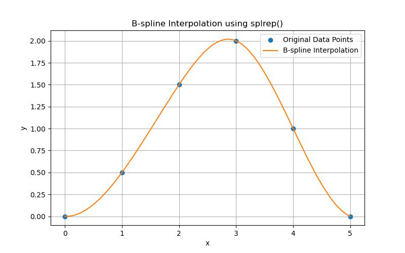
Example

This example shows how to use splrep() to perform B-spline interpolation on a set of data points −

import numpy as np
import matplotlib.pyplot as plt
from scipy import interpolate

# Define the data points (x) and corresponding values (y)
x = np.array([0, 1, 2, 3, 4, 5])
y = np.array([0, 0.5, 1.5, 2.0, 1.0, 0])

# Find the B-spline representation of the curve
# tck contains the knots (t), coefficients (c), and degree (k) of the spline
tck = interpolate.splrep(x, y)

# Generate new x values for interpolation
x_new = np.linspace(0, 5, 100)

# Evaluate the spline at the new x values
y_new = interpolate.splev(x_new, tck)

# Plot the original data points and the interpolated spline curve
plt.figure(figsize=(8, 5))
plt.plot(x, y, 'o', label='Original Data Points')
plt.plot(x_new, y_new, label='B-spline Interpolation')
plt.title('B-spline Interpolation using splrep()')
plt.xlabel('x')
plt.ylabel('y')
plt.legend()
plt.grid(True)
plt.show()

Below is the output of the splrep() function in Scipy −

splev Function

The splev() function is defined as Spline Evaluation which is used to evaluates the spline or its derivatives at given points using the B-spline representation which is obtained from splrep() function. Once we have computed the spline representation using splrep() function then we can use splev() function to interpolate or evaluate the function at new points.

Syntax

Below is the syntax of using the splev() function in scipy −

splev(x_new, tck)

Parameters

Here are the parameters of the splev() function in scipy −

• x_new: array of x-coordinates of the data points.
• tck: The B-spline representation which is the output from splrep() function.
• der(optional): Derivative order with default value as 0 for interpolation.

Example

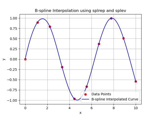
This example shows how the function splev() is used to generate the smooth B-spline curve based on the original data points −

import numpy as np
import matplotlib.pyplot as plt
from scipy.interpolate import splrep, splev

# Sample data points
x = np.linspace(0, 10, 10)
y = np.sin(x)

# Compute the B-spline representation of the data (tck = knots, coefficients, degree)
tck = splrep(x, y)

# New points for evaluating the spline
x_new = np.linspace(0, 10, 100)

# Use splev to evaluate the spline at the new points
y_new = splev(x_new, tck)

# Plot the original data points and the interpolated spline
plt.scatter(x, y, label='Data Points', color='red')
plt.plot(x_new, y_new, label='B-spline Interpolated Curve', color='blue')
plt.title('B-spline Interpolation using splrep and splev')
plt.xlabel('x')
plt.ylabel('y')
plt.grid(True)
plt.legend()
plt.show()

Here is the output of the splev() function in Scipy −

UnivariateSpline

The UnivariateSpline is a convenient class for performing one-dimensional spline interpolation. It fits a spline to a set of data points and allows for smooth interpolation while controlling the smoothing factor. The class also provides flexibility to adjust the degree of the spline and the level of smoothing by making it useful for noisy data or when a smooth and continuous approximation is needed.

Syntax

Below is the syntax of using the UnivariateSpline() class in scipy −

scipy.interpolate.UnivariateSpline(x, y, w=None, bbox=[None, None], k=3, s=None)

Parameters

Following are the parameters of the UnivariateSpline() class in scipy −

• x,y: The data points.
• w: Optional weights for the spline fit.
• k: The degree of the spline with the default value is 3 for cubic spl9ine.
• s: Smoothing factor, if s=0 then the spline will pass through all data points.

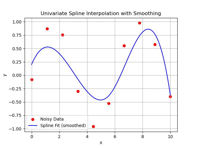
Example

Here in this example we will generate the univariate spline interpolation with the help of UnivariateSpline() class in scipy −

import numpy as np
import matplotlib.pyplot as plt
from scipy.interpolate import UnivariateSpline

# Generate sample data
x = np.linspace(0, 10, 10)
y = np.sin(x) + np.random.normal(0, 0.1, 10)  # Adding noise to the sine function

# Fit a cubic spline to the noisy data
spl = UnivariateSpline(x, y, s=1)  # s is the smoothing factor

# Generate new x values for the smooth spline curve
x_new = np.linspace(0, 10, 100)
y_new = spl(x_new)

# Plot the results
plt.scatter(x, y, color='red', label='Noisy Data')
plt.plot(x_new, y_new, color='blue', label='Spline Fit (smoothed)')
plt.title('Univariate Spline Interpolation with Smoothing')
plt.xlabel('x')
plt.ylabel('y')
plt.legend()
plt.grid(True)
plt.show()

Following is the output of the UnivariateSpline() class in Scipy −

BSpline

In SciPy BSpline is a class used for constructing and evaluating B-spline curves. B-splines can be given as Basis splines which are a generalization of Bzier curves and they provide a way to represent smooth curves through a set of control points. B-splines are widely used in computational geometry, numerical analysis and computer graphics for curve fitting and interpolation.

Syntax

Below is the syntax of using the BSpline() class in scipy −

scipy.interpolate.BSpline(t, c, k, extrapolate=True, axis=0)

Parameters

Following are the parameters of the BSpline() class in scipy −

• t: Array of knot points which sorted in non-decreasing order.
• c: Array of spline coefficients.
• k: Degree of the spline i.e., order.
• extrapolate: Whether to extrapolate for points outside the range of the knots.

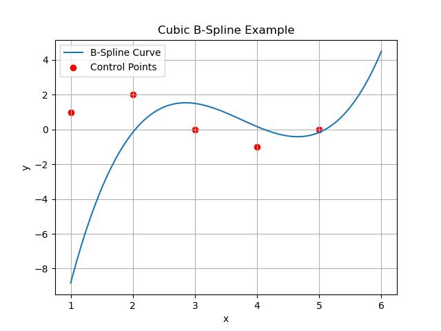
Example

Here in this example we will generate the BSpline interpolation with the help of BSpline() class in scipy −

import numpy as np
import matplotlib.pyplot as plt
from scipy.interpolate import BSpline

# Define the knot vector and coefficients (control points)
knots = [0, 1, 2, 3, 4, 5, 6, 7]  # Knot vector (degree + control points + 1)
coefficients = [1, 2, 0, -1, 0, 2]  # Control points
degree = 3  # Cubic B-spline

# Create the B-spline object
spline = BSpline(knots, coefficients, degree)

# Generate x values for evaluating the spline
x = np.linspace(1, 6, 100)
y = spline(x)

# Plot the B-spline curve
plt.plot(x, y, label='B-Spline Curve')

# Mark the control points
plt.scatter([1, 2, 3, 4, 5], coefficients[:-1], color='red', label='Control Points')

# Add labels, title, grid, and legend
plt.title('Cubic B-Spline Example')
plt.xlabel('x')
plt.ylabel('y')
plt.grid(True)
plt.legend()
plt.show()

Following is the output of the BSpline() class in Scipy −

make_interp_spline

In SciPy the function make_interp_spline() is used to create a B-spline representation for a given set of data points. It fits a smooth B-spline curve to the data points and it is commonly used for 1-D interpolation. Its primarily used when we need a smooth interpolation of data points especially when we want control over the degree of the spline or need to generate smooth curves for plotting.

Syntax

Below is the syntax of using the make_interp_spline() function in scipy −

scipy.interpolate.make_interp_spline(x, y, k=3, bc_type=None, axis=0)

Parameters

Following are the parameters of the make_interp_spline() function in scipy −

• x: The independent variable i.e., 1D array of the x-coordinates of the data points.
• y: The dependent variable i.e., y-values corresponding to x and must be the same shape.
• k: The degree of the spline with the default value is 3 i.e. cubic spline.
• bc_type(optional): Boundary conditions for the spline where we can specify natural, clamped, etc.
• axis: Axis along which to interpolate.

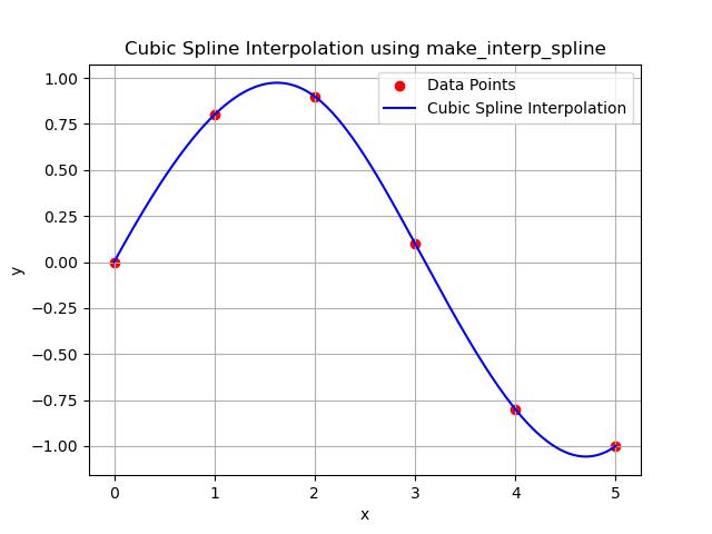
Example

Below is the example which shows how to use make_interp_spline() function for cubic spline interpolation −

import numpy as np
import matplotlib.pyplot as plt
from scipy.interpolate import make_interp_spline

# Define the data points (x, y)
x = np.array([0, 1, 2, 3, 4, 5])
y = np.array([0, 0.8, 0.9, 0.1, -0.8, -1.0])

# Create a new set of x values for interpolation (finer resolution)
x_new = np.linspace(x.min(), x.max(), 300)

# Create the cubic B-spline (k=3 for cubic)
spl = make_interp_spline(x, y, k=3)

# Compute the new y values using the spline
y_new = spl(x_new)

# Plot the original data points and the interpolated curve
plt.scatter(x, y, color='red', label='Data Points')
plt.plot(x_new, y_new, label='Cubic Spline Interpolation', color='blue')
plt.title('Cubic Spline Interpolation using make_interp_spline')
plt.xlabel('x')
plt.ylabel('y')
plt.legend()
plt.grid(True)
plt.show()

Here is the output of the make_interp_spline() function in Scipy −

PchipInterpolator

The PchipInterpolator in SciPy is a class used for Piecewise Cubic Hermite Interpolating Polynomials (PCHIP). It is particularly advantageous for ensuring that the interpolation maintains the shape and monotonicity of the data by making it suitable for applications where preserving the original data's characteristics is crucial.

Syntax

Below is the syntax of using the PchipInterpolator() class in scipy −

PchipInterpolator(x, y, extrapolate=False)

Parameters

Following are the parameters of the PchipInterpolator() class in scipy −

• x: 1D array of the x-coordinates of the data points. Must be strictly increasing.
• y: 1D array of the y-coordinates corresponding to x.
• extrapolate: If this parameter set to True then the interpolator will allow extrapolation beyond the boundaries of x. The default value is False.

Example

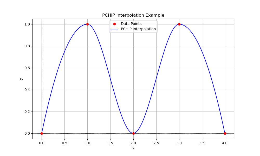
Following is the example which shows how to use PchipInterpolator() class for generating the spline interpolation −

import numpy as np
import matplotlib.pyplot as plt
from scipy.interpolate import PchipInterpolator

# Define sample data points
x = np.array([0, 1, 2, 3, 4])
y = np.array([0, 1, 0, 1, 0])  # Example data with peaks and valleys

# Create the PCHIP interpolator
pchip_interpolator = PchipInterpolator(x, y)

# Generate new x values for interpolation
x_new = np.linspace(0, 4, 100)
y_new = pchip_interpolator(x_new)

# Plot the original data points and the PCHIP interpolated curve
plt.figure(figsize=(10, 6))
plt.scatter(x, y, color='red', label='Data Points', zorder=5)
plt.plot(x_new, y_new, label='PCHIP Interpolation', color='blue')
plt.title('PCHIP Interpolation Example')
plt.xlabel('x')
plt.ylabel('y')
plt.axhline(0, color='black', lw=0.5, ls='--')
plt.axvline(0, color='black', lw=0.5, ls='--')
plt.grid()
plt.legend()
plt.show()

Here is the output of the PchipInterpolator() class in Scipy −