Stationary Wavelet Transform (SWT)

---

---

Stationary Wavelet Transform in SciPy

The Stationary Wavelet Transform (SWT) is a variant of the Discrete Wavelet Transform (DWT) where the scaling and shifting of the wavelet function are done in a way that avoids down-sampling. This results in no loss of information, unlike the DWT which includes down-sampling that may cause some detail loss. SWT is especially useful for applications where high precision in time-frequency analysis is required such as in image processing, de-noising and feature extraction of non-stationary signals.

The Stationary Wavelet Transform of a signal x(t) can be represented as follows −

$\mathrm{W(j, k) = \int_{-\infty}^{\infty} x(t) \psi^* \left( \frac{t - k}{2^j} \right) dt}$

Where −

• x(t) is the input signal.
• (t) is the mother wavelet.
• = 2^j is the scale factor.
• = k is the translation parameter (discrete shifts of the signal).
• W(j, k) represents the wavelet coefficients at scale j and shift k.

Key Properties of SWT

Following are the key properties of the Stationary Wavelet Transform −

• No Down-sampling: Unlike DWT, SWT does not perform downsampling which avoids the loss of detail during decomposition.
• Shift Invariance: The SWT is shift-invariant which means small shifts in the signal do not cause large changes in the wavelet coefficients which makes it suitable for detecting small changes in non-stationary signals.
• Multi-Resolution Analysis: Similar to DWT, SWT allows for multi-resolution analysis by analyzing signals at multiple scales.
• Time-Frequency Localization: SWT provides time-frequency localization by making it useful for non-stationary signal analysis such as speech or biomedical signal processing.

Note:

In SciPy versions 1.15.1 and later the cwt function has been removed from the scipy.signal module. Therefore, for the Continuous Wavelet Transform (CWT) or stationary wavelet transformations alternative libraries such as PyWavelets (pywt) can be used.

Using PyWavelets (pywt)

If we're facing issues with SciPy's DWT function we can use PyWavelets (pywt) which provides efficient implementations of both the DWT and SWT in Python. It supports a wide range of wavelet types and decomposition levels by making it a versatile tool for wavelet analysis.

Basic Example of SWT using PyWavelets

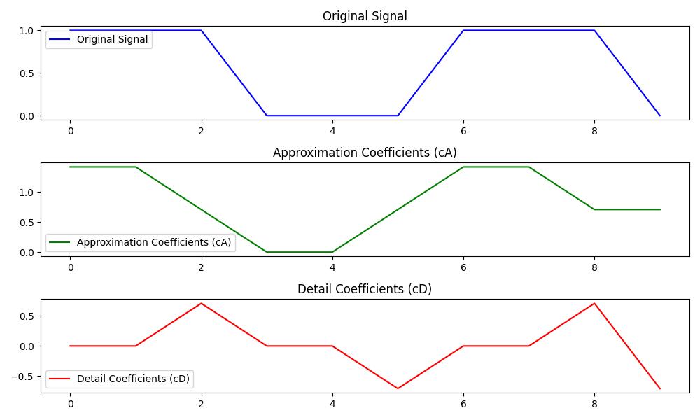
In this example we will perform a 1-level Stationary Wavelet Transform on a simple signal using the Haar wavelet −

import numpy as np
import pywt
import matplotlib.pyplot as plt

# Create a simple signal (a step function for demonstration)
signal = np.array([1, 1, 1, 0, 0, 0, 1, 1, 1, 0])

# Perform 1-level Stationary Wavelet Transform (SWT) using the Haar wavelet
coeffs = pywt.swt(signal, 'haar', level=1)

# Extract the approximation (cA) and detail (cD) coefficients
cA, cD = coeffs[0]

# Plot the original signal, approximation coefficients, and detail coefficients
plt.figure(figsize=(10, 6))

# Plot the original signal
plt.subplot(3, 1, 1)
plt.plot(signal, label="Original Signal", color='blue')
plt.title("Original Signal")
plt.legend()

# Plot the approximation coefficients (cA)
plt.subplot(3, 1, 2)
plt.plot(cA, label="Approximation Coefficients (cA)", color='green')
plt.title("Approximation Coefficients (cA)")
plt.legend()

# Plot the detail coefficients (cD)
plt.subplot(3, 1, 3)
plt.plot(cD, label="Detail Coefficients (cD)", color='red')
plt.title("Detail Coefficients (cD)")
plt.legend()

plt.tight_layout()
plt.show()

Following is the output of the Basic Stationary Wavelet Transform using PyWavelets −

Multi-Level SWT Decomposition using PyWavelets

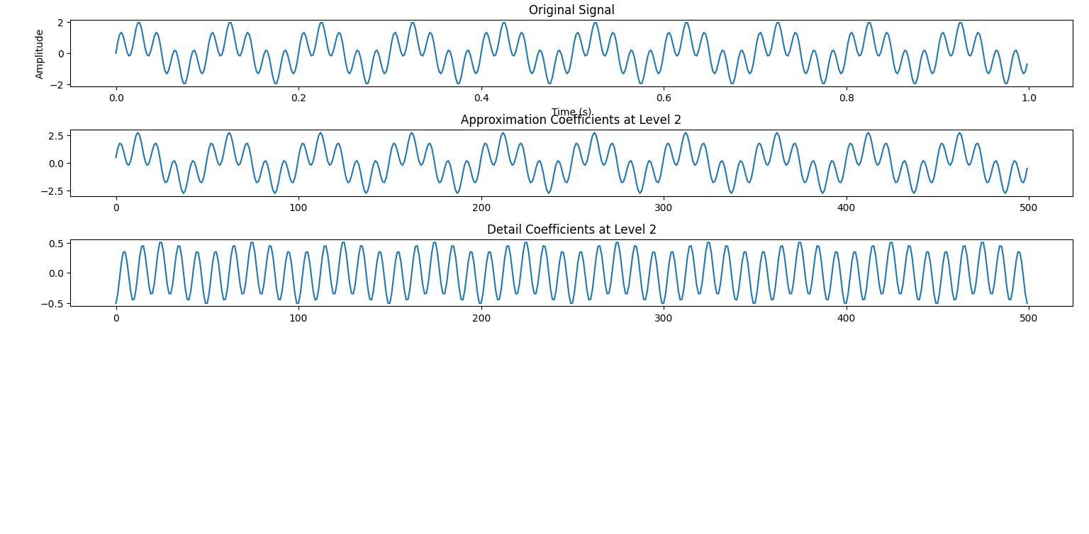
This example shows how to perform multi-level SWT decomposition on a signal using PyWavelets. We will decompose the signal into multiple levels −

import numpy as np
import matplotlib.pyplot as plt
import pywt

# Generate a simple signal (a combination of two sine waves)
t = np.linspace(0, 1, 500, endpoint=False)  # Time vector
signal = np.sin(2 * np.pi * 10 * t) + np.sin(2 * np.pi * 50 * t)  # Signal

# Perform Multi-Level SWT decomposition using 'db1' (Daubechies wavelet)
coeffs = pywt.swt(signal, 'db1', level=2)  # Decompose to 2 levels

# coeffs contains the approximation and detail coefficients at each level
cA2, cD2 = coeffs[1]  # cA2: Approximation at level 2, cD2: Detail at level 2

# Plot the original signal and the decomposition results
plt.figure(figsize=(10, 10))

# Plot the original signal
plt.subplot(5, 1, 1)
plt.plot(t, signal)
plt.title("Original Signal")
plt.xlabel("Time (s)")
plt.ylabel("Amplitude")

# Plot the approximation coefficients at level 2
plt.subplot(5, 1, 2)
plt.plot(cA2)
plt.title("Approximation Coefficients at Level 2")

# Plot the detail coefficients at level 2
plt.subplot(5, 1, 3)
plt.plot(cD2)
plt.title("Detail Coefficients at Level 2")

plt.tight_layout()
plt.show()

Below is the output of the Multi-Level Stationary Wavelet Transform using PyWavelets −

Applications of SWT

The Stationary Wavelet Transform (SWT) is widely used in various fields due to its ability to provide both time and frequency information while preserving the signal's features. Some key applications are as follows −

• Denoising: SWT is often used to remove noise from signals, especially in fields like speech processing, biomedical signal analysis and image processing.
• Compression: SWT can be used for signal and image compression as it provides a compact representation of the data.
• Feature Extraction: SWT is useful for extracting relevant features from signals for machine learning tasks such as classification or pattern recognition.
• Edge Detection: In image processing, SWT can be used for detecting edges and other important features in an image.

Choosing the Right Wavelet for SWT

Just like in DWT by choosing the right wavelet for SWT is essential for capturing the features of the signal being analyzed. Some common wavelets for SWT are as follows −

Wavelet	Best For	Example Use Cases
Daubechies (db)	Smooth signals, multiresolution analysis	Signal denoising, image compression
Symlet	Symmetric signals, efficient approximation	Audio processing, compression
Coiflet	Signals with smooth features, multiresolution	Feature extraction, denoising
Haar	Discontinuous signals, edge detection	Compression, real-time signal analysis