SciPy - Thresholding in Image Segmentation

---

---

Thresholding in image segmentation in SciPy is a fundamental technique used in image processing to separate different regions in an image based on pixel intensity values.

The basic idea is to apply a threshold to an image so that pixels with values above a certain threshold are classified into one group which often called foreground and those below are classified into another group which often called background.

In SciPy library the thresholding image segmentation is often implemented using the scipy.ndimage module along with the other libraries such as Matplotlib and Numpy for image processing. Here in this chapter we will see, thresholding image segmentation in detail.

Types of Thresholding in Image Segmentation

Thresholding is a key method in image processing used to segment an image by converting grayscale values into binary values. There different types of thresholding techniques that cater to various requirements based on the nature of the image as mentioned below −

Global Thresholding

Global thresholding is a simple and effective image segmentation technique where a single threshold value is used to classify pixels into two categories namely, foreground and background. In SciPy global thresholding can be achieved using basic array operations and tools from the scipy.ndimage module.

Following are the steps used to implement the Global thresholding in SciPy −

• Load or create an image.
• Define a global threshold value.
• Apply the threshold by comparing the image pixel values to the threshold.
• Finally, generate a binary mask where pixels above the threshold are classified as foreground True and pixels below are classified as background False.

Example

Here is a complete example of Global Thresholding using NumPy and Matplotlib to implement a Global thresholding operation −

import numpy as np
import scipy.ndimage as ndi
import matplotlib.pyplot as plt

# Create a synthetic grayscale image
np.random.seed(42)
image = np.random.random((100, 100))  # Values between 0 and 1

# Define a global threshold value
threshold_value = 0.5

# Apply global thresholding manually
binary_image = image > threshold_value

# Display the original and binary thresholded images
fig, axes = plt.subplots(1, 2, figsize=(10, 5))

# Original image
axes[0].imshow(image, cmap='gray')
axes[0].set_title("Original Image")
axes[0].axis("off")

# Binary thresholded image
axes[1].imshow(binary_image, cmap='gray')
axes[1].set_title(f"Binary Thresholded Image (T = {threshold_value})")
axes[1].axis("off")

plt.tight_layout()
plt.show()

Below is the output of the Global thresholding of the image segmentation implemented with the help Numpy and Matplotlib libraries −

Otsu's Thresholding

Otsu's Thresholding is a global thresholding technique that determines the optimal threshold value for an image by maximizing the variance between the foreground and background classes. This method assumes that the image has a bimodal histogram i.e., two distinct peaks representing background and foreground.

The main objective of this method is to find the threshold T that minimizes the intra-class variance or equivalently maximizes the inter-class variance.

Example

Otsus Thresholding is not directly implemented in SciPy but we can achieve it by using a combination of SciPy's histogram functionality and NumPy for calculations. Below is the example which gives step-by-step approach of how to implement Otsu's Thresholding in SciPy −

import numpy as np
import scipy.ndimage as ndi
import matplotlib.pyplot as plt

def otsu_threshold(image):
   """
   Computes Otsu's threshold for a grayscale image.
   
   Parameters:
       image (ndarray): Input grayscale image (2D array).
   
   Returns:
       threshold (float): Optimal threshold value.
   """
   # Compute the histogram of the image
   hist, bin_edges = np.histogram(image.ravel(), bins=256, range=(0, 1))
   bin_centers = (bin_edges[:-1] + bin_edges[1:]) / 2
   
   # Total number of pixels
   total_pixels = image.size
   
   # Cumulative sums and cumulative means
   cumulative_sum = np.cumsum(hist)
   cumulative_mean = np.cumsum(hist * bin_centers)
   
   # Global mean
   global_mean = cumulative_mean[-1] / total_pixels
   
   # Between-class variance
   numerator = (global_mean * cumulative_sum - cumulative_mean) ** 2
   denominator = cumulative_sum * (total_pixels - cumulative_sum)
   between_class_variance = numerator / (denominator + 1e-10)  # Add epsilon to avoid division by zero
   
   # Find the maximum of between-class variance
   optimal_idx = np.argmax(between_class_variance)
   optimal_threshold = bin_centers[optimal_idx]
   
   return optimal_threshold
   
# Generate a synthetic grayscale image (random noise for demonstration)
np.random.seed(0)
image = np.random.random((100, 100))

# Apply Otsu's thresholding
optimal_threshold = otsu_threshold(image)
thresholded_image = image > optimal_threshold

# Display the original and thresholded images
fig, ax = plt.subplots(1, 2, figsize=(10, 5))
ax[0].imshow(image, cmap='gray')
ax[0].set_title("Original Image")
ax[0].axis('off')

ax[1].imshow(thresholded_image, cmap='gray')
ax[1].set_title(f"Thresholded Image\n(Otsu's Threshold = {optimal_threshold:.2f})")
ax[1].axis('off')

plt.tight_layout()
plt.show()

Below is the output of implementing the Otsu thresholding −

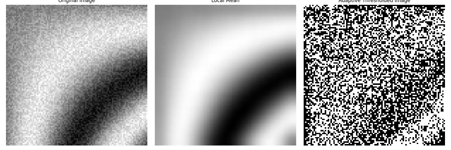
Adaptive Thresholding

Adaptive Thresholding is a thresholding technique where the threshold value varies across the image by depending on local image properties. This method is particularly useful for images with uneven lighting or varying intensity levels where a single global threshold would fail to segment the image properly.

Following are the steps involved in implementing the Adaptive Thresholding −

• Divide the Image into Local Regions: The image is analyzed in small neighborhoods or regions instead of globally.
• Calculate Local Statistics: Compute a local threshold for each pixel based on the statistics e.g., mean or Gaussian-weighted mean of the surrounding region.
• Threshold Each Pixel: Classify pixels as foreground or background based on the locally computed threshold.

Example

Here is an example using SciPy's tools to implement adaptive thresholding using a local mean filter −

import numpy as np
import scipy.ndimage as ndi
import matplotlib.pyplot as plt

# Create a synthetic image with uneven lighting
np.random.seed(0)
x, y = np.meshgrid(np.linspace(0, 1, 100), np.linspace(0, 1, 100))
image = np.sin(10 * x * y) + np.random.random((100, 100)) * 0.5

# Apply a local mean filter
window_size = 15  # Size of the local region
local_mean = ndi.uniform_filter(image, size=window_size)

# Perform adaptive thresholding
thresholded_image = image > local_mean

# Display the results
fig, ax = plt.subplots(1, 3, figsize=(15, 5))
ax[0].imshow(image, cmap='gray')
ax[0].set_title("Original Image")
ax[0].axis('off')

ax[1].imshow(local_mean, cmap='gray')
ax[1].set_title("Local Mean")
ax[1].axis('off')

ax[2].imshow(thresholded_image, cmap='gray')
ax[2].set_title("Adaptive Thresholded Image")
ax[2].axis('off')

plt.tight_layout()
plt.show()

Advanced Adaptive Thresholding Technique

For more advanced adaptive thresholding technique we can use a Gaussian-weighted mean instead of a simple mean. Below is the example of the advanced adaptive thresholding technique −

import numpy as np
import scipy.ndimage as ndi
import matplotlib.pyplot as plt

# Create a synthetic image with uneven lighting
np.random.seed(0)
x, y = np.meshgrid(np.linspace(0, 1, 100), np.linspace(0, 1, 100))
image = np.sin(10 * x * y) + np.random.random((100, 100)) * 0.5

# Apply a local Gaussian filter
sigma = 5  # Standard deviation for Gaussian kernel
local_gaussian_mean = ndi.gaussian_filter(image, sigma=sigma)

# Perform adaptive thresholding
thresholded_image_gaussian = image > local_gaussian_mean

# Display results
fig, ax = plt.subplots(1, 2, figsize=(10, 5))
ax[0].imshow(local_gaussian_mean, cmap='gray')
ax[0].set_title("Local Gaussian Mean")
ax[0].axis('off')

ax[1].imshow(thresholded_image_gaussian, cmap='gray')
ax[1].set_title("Gaussian Adaptive Thresholded Image")
ax[1].axis('off')

plt.tight_layout()
plt.show()

Below is the output of the advanced adapative filtering −