SciPy - Top-Hat Filters

---

---

The Top-Hat filter in SciPy is a morphological operation designed to highlight specific intensity features in an image. It is particularly useful for detecting and enhancing small, localized features that are either brighter or darker than their surroundings. There are two primary types of top-hat filters as follows −

• White Top-Hat Filter
• Black Top-Hat Filter

Now, let's see each type of the Top-Hat Filters in detail −

White Top-Hat Filter

The White Top-Hat Filter is a morphological operation that extracts small bright features from an image that are smaller than the structuring element.

It is often used to enhance bright details, remove uneven background illumination or highlight specific regions of interest. The White Top-Hat filter is mathematically defined as follows −

WhiteTop-HatImage = OriginalImageOpenedImage

A morphological operation that consists of erosion followed by dilation. It smooths the image by removing small bright regions that do not fit within the structuring element.

Subtracting the opened image from the original image enhances the bright regions that were removed during the opening process.

Creating/Implementing White Top-Hat Filter

The structuring element i.e., a kernel defines the size and shape of the features to extract. The bright regions smaller than the structuring element are isolated because the opening operation removes bright regions smaller than the structuring element and subtraction restores these regions while suppressing the larger-scale structures.

In SciPy the White Top-Hat Filter can be implemented by the function scipy.ndimage.white_tophat().

Syntax

Following is the syntax of the function scipy.ndimage.white_tophat() which is used to extract small bright features from an image −

scipy.ndimage.white_tophat(
   input, 
   size=None, 
   footprint=None, 
   structure=None, 
   output=None, 
   mode='reflect',
   cval=0.0, 
   origin=0
)

Following are the parameters of the scipy.ndimage.white_tophat() function −

• input: The input image or array i.e., grayscale or binary.
• size: This parameter specifies the size of a square structuring element.
• footprint: A binary array that defines the shape of the structuring element.
• structure: It specifies the exact structuring element and overrides size and footprint.
• mode: This determines how image boundaries are handled.
• cval: The constant value used when mode='constant'.
• origin: This parameter controls the position of the structuring element relative to the current pixel.

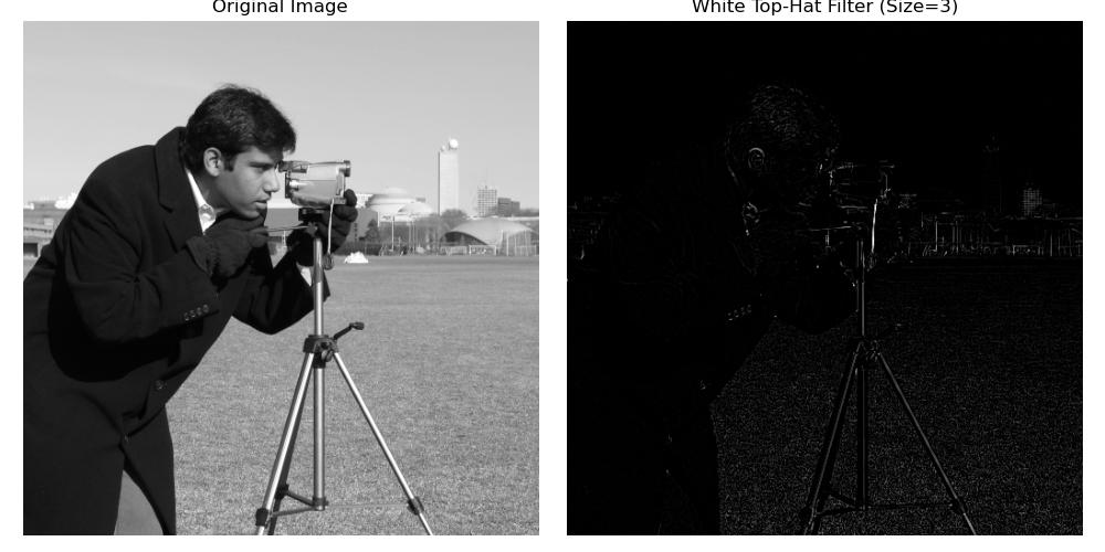
White Top-Hat Filter with Default Structuring Element

Following is the basic example of the function scipy.ndimage.white_tophat(), in which we will apply the white top-hat filter using the default structuring element i.e., a 3x3 square to a sample image (camera) from skimage.

import numpy as np
import matplotlib.pyplot as plt
from scipy.ndimage import white_tophat
from skimage.data import camera

# Load the sample image
image = camera()

# Apply the white top-hat filter with the default structuring element (3x3 square)
result = white_tophat(image, size=3)

# Plot the original and filtered images side by side
plt.figure(figsize=(12, 6))

# Original Image
plt.subplot(1, 2, 1)
plt.title("Original Image")
plt.imshow(image, cmap='gray')
plt.axis('off')

# White Top-Hat Filter Result
plt.subplot(1, 2, 2)
plt.title("White Top-Hat Filter Result")
plt.imshow(result, cmap='gray')
plt.axis('off')

plt.tight_layout()
plt.show()

Here is the output of the function scipy.ndimage.white_tophat() −

White Top-Hat Filter with Varying the Size Parameter

The size parameter in the white top-hat filter controls the size of the structuring element used for the morphological opening operation. By changing this parameter we can adjust the scale of the features that we want to enhance i.e., the size of the small bright features where we want to isolate. Here is the example which varies the size parameter as per requirement −

import numpy as np
import matplotlib.pyplot as plt
from scipy.ndimage import white_tophat
from skimage.data import camera

# Load the example image
image = camera()

# Apply white top-hat filter with small structuring element (size=5)
result_small = white_tophat(image, size=5)

# Display results
plt.figure(figsize=(10, 5))
plt.subplot(1, 2, 1)
plt.title("Original Image")
plt.imshow(image, cmap='gray')
plt.axis('off')

plt.subplot(1, 2, 2)
plt.title("White Top-Hat (size=5)")
plt.imshow(result_small, cmap='gray')
plt.axis('off')
plt.tight_layout()
plt.show()

Here is the output of the function scipy.ndimage.white_tophat() which varies the size −

Black Top-Hat Filter

The Black Top-Hat Filter also called as Bottom Hat Filter, which is a morphological operation that is used to extract small dark features from an image. It works in the opposite manner of the White Top-Hat Filter, in which it highlights small bright regions.

The Black Top-Hat filter helps to isolate small dark regions i.e., dark spots against a brighter background. The mathematical definition for the Black Top-Hat Filter can be given as follows −

BlackTop-Hat = ClosedImage  OriginalImage

Where −

• Closing: The closing operation consists of dilation followed by erosion which smoothens the image by filling small holes in bright regions.
• Subtracting the original image from the closed image helps to isolate small dark regions that were enhanced by the closing operation.

In Scipy we have a function namely, scipy.ndimage.black_tophat() to implement the Black Top-Hat Operation −

Syntax

Following is the syntax of the function scipy.ndimage.black_tophat() to perform the Black Top-Hat Operation on the image −

scipy.ndimage.black_tophat(
   input, 
   size=None, 
   footprint=None, 
   structure=None, 
   output=None, 
   mode='reflect', 
   cval=0.0, 
   origin=0
)

Here are the parameters of scipy.ndimage.black_tophat() function −

• input: The input image or array, i.e., grayscale or binary.
• size: This parameter specifies the size of a square structuring element.
• footprint: A binary array that defines the shape of the structuring element.
• structure: It specifies the exact structuring element and overrides 'size' and 'footprint'.
• output: The array to store the result of the filter. If not specified then a new array will be created.
• mode: This determines how image boundaries are handled and the modes are such as 'reflect', 'constant', 'nearest', etc.
• cval: The constant value used when mode='constant' to pad the boundaries.
• origin: This parameter controls the position of the structuring element relative to the current pixel.

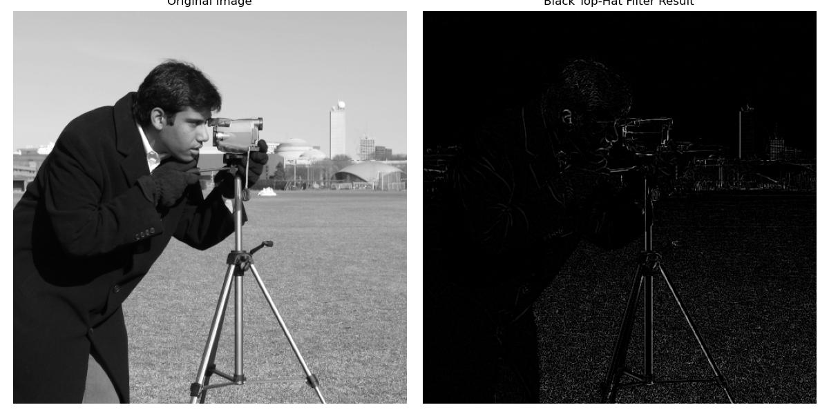
Black Top-Hat Filter with Default Structuring Element

Following is the example of the function scipy.ndimage.black_tophat() in which we'll apply the Black Top-Hat filter using the default structuring element i.e., a 3x3 square to the sample image (camera from skimage) −

import numpy as np
import matplotlib.pyplot as plt
from scipy.ndimage import black_tophat
from skimage.data import camera

# Load the sample image
image = camera()

# Apply the black top-hat filter with the default structuring element (3x3 square)
result = black_tophat(image, size=3)

# Plot the original and filtered images side by side
plt.figure(figsize=(12, 6))

# Original Image
plt.subplot(1, 2, 1)
plt.title("Original Image")
plt.imshow(image, cmap='gray')
plt.axis('off')

# Black Top-Hat Filter Result
plt.subplot(1, 2, 2)
plt.title("Black Top-Hat Filter Result")
plt.imshow(result, cmap='gray')
plt.axis('off')

plt.tight_layout()
plt.show()

Following is the output of the basic example implemented using scipy.ndimage.black_tophat() function −

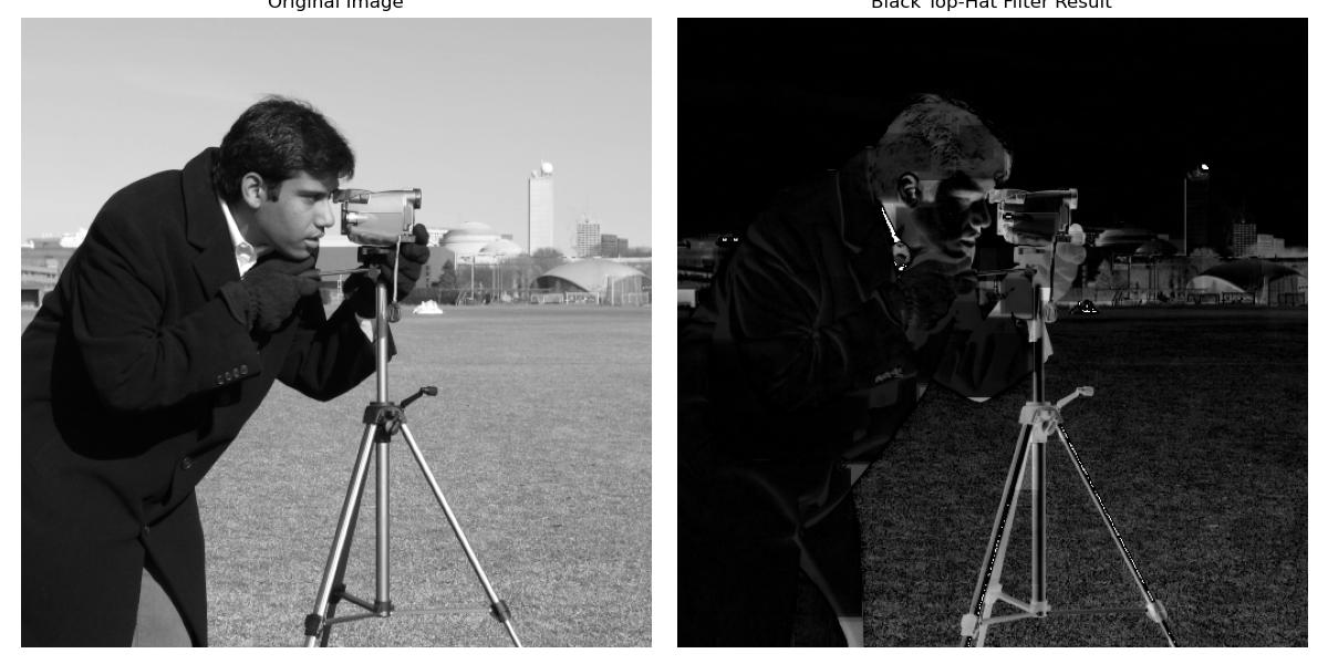
Black Top-Hat Filter with a Custom Structuring Element

In this example we'll use a disk-shaped structuring element with a radius of 10 pixels to extract dark spots using a custom shape −

import numpy as np
import matplotlib.pyplot as plt
from scipy.ndimage import black_tophat
from skimage.morphology import disk
from skimage.data import camera

# Load the sample image
image = camera()

# Define a disk-shaped structuring element with radius 10
structuring_element = disk(10)

# Apply the black top-hat filter with the custom structuring element
result = black_tophat(image, structure=structuring_element)

# Plot the original and filtered images side by side
plt.figure(figsize=(12, 6))

# Original Image
plt.subplot(1, 2, 1)
plt.title("Original Image")
plt.imshow(image, cmap='gray')
plt.axis('off')

# Black Top-Hat Filter Result
plt.subplot(1, 2, 2)
plt.title("Black Top-Hat Filter Result")
plt.imshow(result, cmap='gray')
plt.axis('off')

plt.tight_layout()
plt.show()

Following is the output of the example implemented using scipy.ndimage.black_tophat() function with disk structuring element −