Scipy Triple Integration (tplquad)

---

---

---

Triple Integration in SciPy

In SciPy Triple Integration can be performed using the tplquad() function from the scipy.integrate module. This function allows us to compute the integral of a function of three variables over a specified region in three-dimensional space. The integral is computed iteratively for each variable following the specified bounds.

The triple integral of a function f(x, y, z) over a three-dimensional region defined by the limits can be expressed mathematically given as follows −

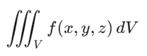
Where −

• V is the three-dimensional region over which the integration is performed.
• dv is the volume element which is in Cartesian coordinates is expressed as dv = dxdydz and f(x, y, z) is the function being integrated.

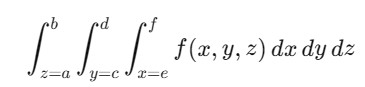
The limits of integration can vary based on the region v. If the limits are constant then the triple integral can be written as follows −

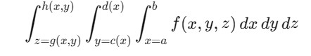
If the limits are functions of one another then the triple integral can be given as −

Syntax

Following is the syntax for the tplquad() function of scipy.integrate module can be given as follows −

scipy.integrate.tplquad(func, a, b, gfun, hfun, vfun, wfun, args=(), epsabs=1.49e-08, epsrel=1.49e-08)

Parameters

Here are the parameters for the tplquad() function of scipy.integrate module −

• func: The function to be integrated which takes three arguments (z, y, x).
• a: The lower limit of integration for the outer integral (x).
• b: The upper limit of integration for the outer integral (x).
• gfun: A function that returns the lower limit of integration for the middle integral (y) as a function of x.
• hfun: A function that returns the upper limit of integration for the middle integral (y) as a function of x.
• vfun: A function that returns the lower limit of integration for the inner integral (z) as a function of x and y.
• wfun: A function that returns the upper limit of integration for the inner integral (z) as a function of x and y.
• args (optional): Extra arguments to pass to func.
• epsabs: Absolute tolerance for the integration where default value is 1.49e-08.
• epsrel: Relative tolerance for the integration where default value is 1.49e-08.

Example of Triple Integration

Below is the example of calculating the triple integral of the function f(x, y, z) = x * y * z over the region defined by

• 0 x 1
• 0 y x
• 0 z y

import scipy.integrate as integrate

# Define the integrand function: f(x, y, z) = x * y * z
def integrand(z, y, x):
    return x * y * z

# Perform triple integration using scipy.integrate.tplquad
result, error = integrate.tplquad(
   integrand, 
   0, 1,              # Limits for x
   lambda x: 0,       # Lower limit for y
   lambda x: x,       # Upper limit for y
   lambda x, y: 0,    # Lower limit for z
   lambda x, y: y     # Upper limit for z
)
# Print the result and estimated error
print("Result of the triple integration:", result)
print("Estimated error:", error)

Following is the output of the triple integration done using the function tplquad() of scipy.integrate −

Result of the triple integration: 0.020833333333333336
Estimated error: 5.4672862306750106e-15

Handling Infinite Limits

We can also handle infinite limits using scipy.inf or -scipy.inf. This allows us to compute integrals over unbounded regions effectively.

Example

Below is an example of integrating the function f(x, y, z) = e^{-(x2 + y2 + z2)} over the region where x, y, z range from 0 to infinity:

import numpy as np
import scipy.integrate as integrate

# Define the function to integrate: f(x, y, z) = exp(-(x^2 + y^2 + z^2))
def integrand(z, y, x):
    return np.exp(-(x**2 + y**2 + z**2))

# Perform triple integration with infinite limits
result, error = integrate.tplquad(integrand, 
                                   0, np.inf,               # Limits for x
                                   lambda x: 0,             # Lower limit for y
                                   lambda x: np.inf,        # Upper limit for y
                                   lambda x, y: 0,          # Lower limit for z
                                   lambda x, y: np.inf)     # Upper limit for z

# Print the result and estimated error
print("Result of the triple integration:", result)
print("Estimated error:", error)

Following is the output of handling the Infinite limits when calculating the triple integration −

Result of the triple integration: 0.6960409996034802
Estimated error: 1.4884526702265109e-08

Error Tolerance

The tplquad() function allows us to control error tolerance with the epsabs and epsrel parameters. These parameters define the desired accuracy of the integration results.

Example

Heres an example of calculating the triple integral with specified error tolerances −

import numpy as np
import scipy.integrate as integrate

# Define the function to integrate: f(x, y, z) = exp(-(x^2 + y^2 + z^2))
def integrand(z, y, x):
    return np.exp(-(x**2 + y**2 + z**2))

# Perform triple integration with custom error tolerances
result, error = integrate.tplquad(integrand, 
                                   0, np.inf,               # Limits for x
                                   lambda x: 0,             # Lower limit for y
                                   lambda x: np.inf,        # Upper limit for y
                                   lambda x, y: 0,          # Lower limit for z
                                   lambda x, y: np.inf,     # Upper limit for z
                                   epsabs=1e-10, epsrel=1e-10)  # Custom tolerances

# Print the result and estimated error
print("Result of the triple integration:", result)
print("Estimated error:", error)

Following is the output of handling the error tolerance while performing the triple integration −

Result of the triple integration: 0.6960409996039614
Estimated error: 9.998852642787021e-11

Complex Functions

When dealing with complex functions we have to split the real and imaginary parts and perform separate integrals for each. This is similar to how double integrals are handled.

Example

Heres an example of calculating the triple integral of a complex function f(x, y, z) = e^{-(x2 + y2 + z2)} + i.sin(x + y + z) −

import numpy as np
from scipy.integrate import nquad

# Define the real part of the function
def real_function(x, y, z):
    return np.exp(-(x**2 + y**2 + z**2))

# Define the imaginary part of the function
def imaginary_function(x, y, z):
    return np.sin(x + y + z)

# Define the limits for each variable (0 to 1 for this example)
limits = [[0, 1], [0, 1], [0, 1]]  # Integration limits for x, y, z

# Perform the triple integration for the real part
real_result, real_error = nquad(real_function, limits)

# Perform the triple integration for the imaginary part
imaginary_result, imaginary_error = nquad(imaginary_function, limits)

# Combine the results into a complex number
result = real_result + 1j * imaginary_result

# Print the results
print(f"Real Part Integral Result: {real_result}, Error Estimate: {real_error}")
print(f"Imaginary Part Integral Result: {imaginary_result}, Error Estimate: {imaginary_error}")
print(f"Combined Integral Result: {result}")

Here is the output of calculating the triple integration of complex functions using tplquad() in scipy −

Real Part Integral Result: 0.4165383858866382, Error Estimate: 8.291335287314424e-15
Imaginary Part Integral Result: 0.8793549306454008, Error Estimate: 1.0645376503904486e-14
Combined Integral Result: (0.4165383858866382+0.8793549306454008j)

Finally we can say the tplquad() function in SciPy provides a powerful and flexible tool for performing triple integrals over various domains.

By specifying functions for the limits and integrating a wide range of functions we can efficiently compute complex integrals with high accuracy.